
With the increase in air traffic over the past decades, the reduction of aircraft noise is one of the major challenges facing stakeholders. Flight operating conditions that decrease noise may possibly increase the fuel consumption of aircraft, which is an important factor in airline cost management. In this paper, we propose a methodology to support flight path planning with the aim of optimising both perceived noise and fuel consumption. We decompose an aircraft flight trajectory into surface and altitude paths to model relevant air transportation constraints. The shortest path for the surface projection is found using Dubins path method and an improved A* algorithm, which considers guide points according to the flight destination, runway angles, spatial separation of aircraft near the airport, population distribution, and steering motion. The altitude path is optimised for low-perceived noise and low-fuel consumption, which is determined by solving the longitudinal governing equations of motion of flight using the distance computed from this surface path. A modified nondominated sorting genetic algorithm II for discrete optimisation is developed to obtain Pareto fronts of the optimum altitude paths with reduced computational effort. The methodology is demonstrated by simulating flights departing from Hong Kong International Airport to two compulsory air-traffic-service reporting points. The results are then compared with Quick Access Recorder data and Standard Instrument Departure (SID) tracks. Although certain factors in air transportation that affect departure path planning, such as weather patterns and air traffic mix, are not considered in this method, the resulting surface path exhibits a close similarity with SID tracks. The resulting Pareto fronts of the altitude path exhibit reductions in fuel consumption and perceived noise levels. The trade-offs between fuel consumption and perceived noise levels are also discussed based on the relevant flight physics for the different routes.
I. Introduction
The rapid growth of air traffic and the increased aircraft noise as a consequence has led to adverse effects on residents living near airports, including sleep disturbance and stress-related health effects [1]. This issue can be addressed either through aircraft design or air traffic management, among other approaches [2]. For aircraft design, new airframes and engines can be designed to reduce the source noise of an aircraft [3]. Since the 1980s, further noise reduction by changing the aircraft design has been very difficult to achieve without affecting operating costs [4]. For air traffic management, the flight routes can be altered to reduce perceived noise, e.g., by increasing the climb rate after take-off. This approach is more "practical", but does not address the issue of reducing source noise and may potentially increase fuel consumption [5]. The perceived noise and fuel consumption are dependent on changes in engine power settings and distance between the aircraft and the observer in a complex manner [6]. Fuel consumption is an important factor directly related to airline revenues and is also proportional to air pollution and greenhouse gas emissions [7]. Hence, it must be considered simultaneously with the perceived noise when optimising operating conditions during flight.
In practice, the departure paths around airports are guided by Standard Instrument Departure (SID) procedures. SID is the coded flight procedure from the point where the departure route begins to the first fix/facility/waypoint of the en-route phase, which varies across airports [8]. The civil aviation authorities of each country design and publish SID in accordance with the design criteria specified in ICAO Doc. 8168 [8], taking into account factors including, but not limited to, runway angles, terrain, obstacle avoidance, aircraft performance, airspace management, and environmental concerns. According to the Civil Aviation Department (CAD) in Hong Kong, the design procedure starts with a preliminary discussion with stakeholders, including the operators/pilots and air traffic controllers. The flyability of the preliminary tracks under different weather and loading scenarios is then tested in flight simulations and subsequently validated by actual flight tests before publication. Computational optimisation research to refine the process of departure path design with quantitative standards has been conducted by Zachary et al. [9], Prats et al. [10], Torres et al. [11], Ho-Huu et al. [12], Filippone et al. [13], and Thomas and Hansman [14]. These studies proposed multi-objective or multilevel departure path planning methodologies considering both fuel consumption and perceived noise level. However, to the best of our knowledge, these studies do not take into account the combined effect of guide points according to flight destinations (i.e., the compulsory Air Traffic Service [ATS] reporting points considered in this study), obstacle restrictions provided by the Aeronautical Information Publication (AIP), and population and topological information. Some of them do not compare their results against existing SID tracks or flight data either. To address these gaps, this paper presents a departure path planning methodology for low-noise and low-fuel consumption that simultaneously considers all of the above factors.
Multi-objective flight path optimisation with many constraints is computationally expensive [15]. To find a Pareto optimal set of solutions considering multiple, diverse constraints while maintaining a certain amount of computational efficiency, this study makes three contributions. The first contribution is decomposing four-dimensional trajectory planning (three-dimensional space plus time) into two subproblems: 1) planning the shortest path projected on Earth's surface considering mainly geography/topography-related constraints, such as no-fly zones, population-based non-preferable areas with runways, and path angle constraints, and 2) planning velocity-varying altitude paths along the shortest path to optimise accumulated perceived noise level and fuel consumption considering vertical flight performance-related constraints. Trajectory planning using the decomposition method was first introduced by Kant and Zucker [16] to reduce the complexity of trajectory planning problems in dynamic environments with stationary and moving obstacles. Their study proposed a sequential planning scheme in which the first step solves a purely spatial optimisation problem for the path, and the second step solves a time-dependent problem for the velocity on the path generated from the first step. It is emphasised that the initial spatial solution is not affected by the subsequent temporal solution. The flight trajectory decomposition method proposed by Hartjes and Visser [17], however, considered velocity coupling in two subproblems, lateral and vertical path planning. The airspeed of an aircraft obtained from vertical path planning constrains the turning radii in the lateral path planning. The paths in their study were determined after prescribing a fixed number of segments from origin to destination. The types of segments in lateral path planning were limited to straight-line and constant-radius turning segments. The vertical path planning was restricted by fixed altitude and airspeed at the terminal position. The trajectory decomposition presented in this paper has no restrictions on the type or number of path segments; the terminal altitude is used as one of the design variables bounded by AIP limits. These formulations enable wide exploration of the design space with the benefit of reduction in complexity of multi-objective optimisation by the decomposition approach. The four-dimensional trajectory planning in this study is decomposed into surface and altitude paths, which are coupled by the arc length of the surface path. After the shortest path problem to minimise this arc length is solved in surface path planning, fuel consumption and accumulated perceived noise level in altitude path planning are evaluated. A turning radius constraint, which can be possibly neglected by not applying velocity coupling, is independently considered in the surface path planning.
The second contribution of this research is a novel methodology for the shortest path planning that enables consideration of non-preferable regions together with no-fly zones and path angle constraints. Most offline path planning in literature has considered paths avoiding static obstacles, which are topographic and geographic restrictions that a trajectory cannot pass over [18–21]. In our method, we introduce a degree of non-preference in addition to static obstacles. The non-prefer-ence is evaluated for the entire domain of path planning, and the solution tends to alter the path to regions in which this degree is low. The degree of non-preference in this study is determined based on population distribution; hence we deem non-preference to be high near regions where the density of people who may be affected by aircraft noise is high. We represent this non-preference as repulsive forces of a potential field, which is one type of path planning method. Path planning methods are broadly classified into four types [22]: 1) grid-based graph [18,23], 2) sampling-based method [19,20], 3) potential field [21,24], and 4) optimal control theory [25,26]. Grid-based graph methods solve the shortest path problem over a grid defined between an origin and a target. The convergence of the solution is guaranteed, but the solution can be unphysical depending on the shape of the grid [27]. Sampling-based methods, on the other hand, determine the optimal path from a sample space instead of searching on a preconstructed grid [28]. The method provides results with low computational time, but it may generate an inefficient path for planning in a large domain [29]. Potential field methods simulate an object moving toward a target, which is modelled as a region with an attractive force, while obstacles are modelled as regions with repulsive forces [30]. They are suitable in real-time path planning for their low computational time, but may converge at local minima [31]. Optimal control methods optimise a specific performance index based on governing equations of motion. The resulting path is physically reasonable, but the convergence of the solution is not always guaranteed [32]. In recent approaches, combinations of these methods have been formulated to compensate for their respective shortcomings [33]. For example, the grid-based graph and the sampling-based methods are combined to smooth the unphysical routes generated by the former due to the grid specifications. In this research, we combine the four methods for fast and physically reasonable surface path planning to model air transportation constraints. First, Dubins path, an optimal control method, is applied to the initial part of the SID procedure close to the runway. As runway angles and the spatial separation requirements of flight routes tightly restrict the take-off flight path, Dubins paths are introduced to model this take-off flight path planning with initial and terminal heading constraints. Second, a population-aware A* algorithm with steering constraints from the end of Dubins path to the target is proposed. This algorithm incorporates potential field and sampling-based methods into a grid-based graph method. Our method is derived from the A* algorithm, a popular shortest-path finding grid-based graph method, for its completeness, ease of modification, and fast computation. As mentioned above, the potential field based on the population density is incorporated into the A* algorithm so that the shortest path can be planned considering populations in quantifying the perceived noise level. Following sampling-based methods, our method searches a sample space to perform path smoothing. Path angle constraints are introduced in this sample space search to help deal with factors relevant to aircraft manoeuvrability. Such a combination of methods makes our approach more realistic and relevant to real-world applications.
The last contribution is altitude path determination via multi-objective optimisation with integer programming. After the surface path planning, the altitude paths along the surface path that minimise the accumulated perceived noise and fuel consumption are computed. As fuel consumption and accumulated perceived noise levels are coupled, the solution that minimises both does not result in an optimum path without predefined preferences [6]. The solutions are represented as a Pareto front set, which shows the trade-off sensitivities for decision-making processes. The Pareto front set is mainly obtained using evolutionary algorithms if the number of design variables is small and the objective function profile is not exactly known, so continuity cannot be guaranteed. Multi-objective optimisation using evolutionary algorithms is known to suffer from high computational time [17], and it is difficult to determine convergence. To address this issue, we limit the design variables to integers with prescribed uniform intervals, where the interval is reasonably chosen based on the physical meaning of each variable. The restriction to this domain avoids function evaluations for relatively insignificant variations, e.g., altitude changes within one metre. Furthermore, under this setting, we can rationally set the number of function evaluations in evolutionary algorithms since the size of the design space can be estimated by the finite number of design variables.
In summary, we developed a multi-objective flight path optimisation methodology that considers various practical constraints to model air transportation operations during departure. The decomposition of four-dimensional flight path planning into sequential surface and altitude path planning procedures is introduced to reduce computational time. Surface path planning that considers guide points according to flight destination, static obstacles, runway angles, spatial separation near airports, non-preferable regions based on population distribution, and steering constraints is proposed. Altitude path planning with integer programming is developed for efficient computation. It is acknowledged that the developed methodology still has limitations in modelling certain factors in air transportation that affect departure path planning, such as weather patterns and air traffic mix. We implement our methodology for the path planning of an aircraft departing from Hong Kong International Airport (HKIA) to two different destinations. The results exhibit a close similarity with SID tracks by graphical comparison. As such, the method presented in this paper can still provide a quantitative basis to assist in decision-making processes for determining departure flight paths with low-fuel consumption and low-perceived noise while considering air transportation constraints.
The structure of this paper is as follows. Section II details the methodology of flight path planning, multi-objective optimisation, fuel consumption, and noise prediction models. Section III presents the results and discussion of the developed methodology applied to two origin-destination pairs and compares them to actual flight trajectory data with validation. Section IV summarises the findings and concludes the study.
II. Methodology
This section introduces a flight path planning methodology that reduces perceived noise levels and fuel consumption. The flight path refers to the trajectory of an aircraft, which is represented as surface coordinates and altitude, following the World Geodetic System 1984 convention [34]. In this study, the flight path is decomposed into surface and altitude paths. Surface path refers to the position of the aircraft projected on a plane onto Earth's surface, and altitude path refers to the position of the aircraft projected on a plane with arc length (the accumulated travel distance on Earth's surface) and altitude as coordinates. The surface and altitude path are coupled with the accumulated travel distance, which is first minimised in the surface path planning. Once the shortest surface path is generated under given constraints of flight regulations, steering angles, number of residents in the area, the altitude path problem is solved for optimal low-perceived noise and low-fuel consumption levels according to changes in the altitude at a fixed distance corresponding to the arc length on the surface. Section II.A details the surface path planning method, and Sec. II.B details the altitude path planning method.
A. Surface Path Planning
An aircraft must contact the Air Traffic Control (ATC) tower at a location designated by Aeronautical Information Services (AIS) when entering or leaving the airspace of any country; this location is called the compulsory ATS reporting point. This section details the surface path planning method from take-off to the ATS reporting point. The developed surface path planning method sequentially performs path planning in two phases: initial and subsequent departures. The initial departure phase begins from the runway to a fixed point, which is on a direct-to-fix leg described in AIP [35]. The designated endpoint of the first direct-to-fix leg near an airport accounts for lateral spatial separation of aircraft for the ATC to manage air traffic during departures for the respective runways at similar times. The subsequent departure phase is a flight phase from this fixed point to a compulsory ATS reporting point.
Section II.A.1 describes the methodology used to computationally model the surface paths. Section II.A.2 details the method to address high-elevation areas as well as prohibited, restricted, and dangerous areas defined by AIP‡. Section II.A.3 describes surface path planning for the initial departure phase. Sections II.A.4 and II.A.5 detail the surface path planning methodology for the subsequent departure phase considering population distributions and path smoothing with steering constraints.
1. Grid Generation
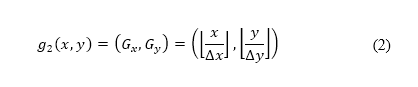
The projection of the aircraft trajectory onto the surface of Earth is mapped to a grid for modelling overall surface path planning. This grid is generated based on geographic information. First, we transform the geographic information represented in geodetic coordinates into Cartesian coordinates. We define a boundary for the path planning region by specifying four latitude-longitude points  on Earth's surface such that the enclosed region covers the departure airport and the target compulsory ATS reporting point. The geodetic coordinates are transformed to Cartesian coordinates
  . Let
. Let  be the coordinate transformation from geodetic coordinates to Cartesian coordinates, defined as
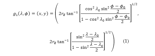
where  is the radius of Earth, and
  and
and  denote the latitude and longitude of the lower-left corner of the boundary respectively. The coordinate transformation
  is derived from Haversine distances [36] of the current position
  to
to  and
and  . Second, we discretise this Cartesian space and define a mapping to a grid. The axes of the Cartesian domain are discretised with uniform intervals
  and
and  to generate the grid points. Let
  be the coordinate transformation of Cartesian coordinates to the grid point
  , defined as
Let  be the representative, finite domain for the surface path trajectory optimisation problem. Let
  be the restriction of
  to integers, which defines the domain of the grid. An air-transportation-regulated constraint, which is expressed in terms of geodetic coordinates, is mapped to the grid by the composition of functions and
  , defined as
As is not invertible, the notation  presented subsequently denotes its right inverse, which is the inclusion map to integer coordinates as a subset of .
2. Obstacle Constraints
The generated surface path takes any no-fly zones into account. No-fly zones are areas over which the aircraft must not fly, such as prohibited, restricted, and dangerous areas designated in AIP, and areas where the ground elevation is higher than 500 m above sea level. Figure 1 shows no-fly zones in Hong Kong airspace and its representation on the grid. In our method, we treat no-fly zones as areas with obstacle constraints. The obstacles shown on the left-hand side of Fig 1 are classified into four types: point obstacles, points with radii, points on the vertices of the regional boundary, and map boundary. The point obstacles refer to areas where the ground elevation is higher than 500 m above sea level, which are shown as red dots. The data are locations , using information extracted from Google Earth§ with point sampling; they are transformed to Cartesian coordinates by . The points with radii and the points on the vertices of the regional boundary, presented as blue lines on the left-hand side of Fig 1, correspond to prohibited, restricted, and dangerous areas listed in AIP. These points are also transformed by and then applied to geometric equations, such as those corresponding to a circle and a line segment, to determine the points included within regions enclosed by the blue lines presented in the figure. To constrain the flight path within the grid, the map boundary is also treated as a restricted region by modelling it as an obstacle. Let  be the location of an obstacle. Let
  be the neighbourhood of
  such that
  . This neighbourhood represents the region surrounding the obstacle, which we define as the obstacle region. Let
  be an indicator function that represents the evaluation of constraint violation. The following defines the constraint violation indicator for obstacle regions:
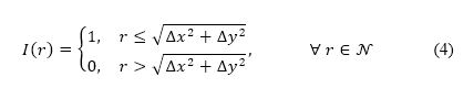
where the distance  from a point
  to obstacle
  is determined by the Euclidean norm
 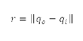 . The constraint violations of the aforementioned four obstacle types are evaluated by Eq. (4) and their locations mapped to the grid by g. The obstacle regions generated by this procedure are depicted in dark blue on the right-hand side of Fig 1, while the white region depicts the permitted region. The surface path is constrained by preventing the aircraft from passing through these restricted regions on the grid.
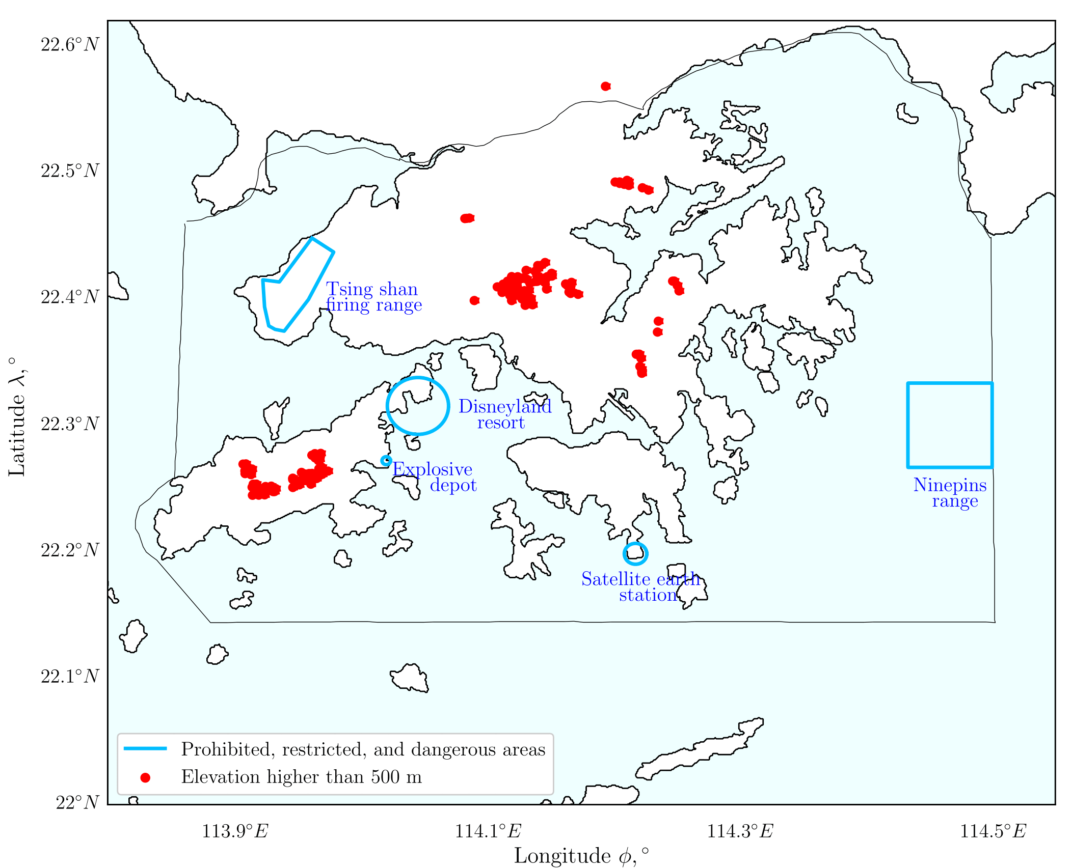
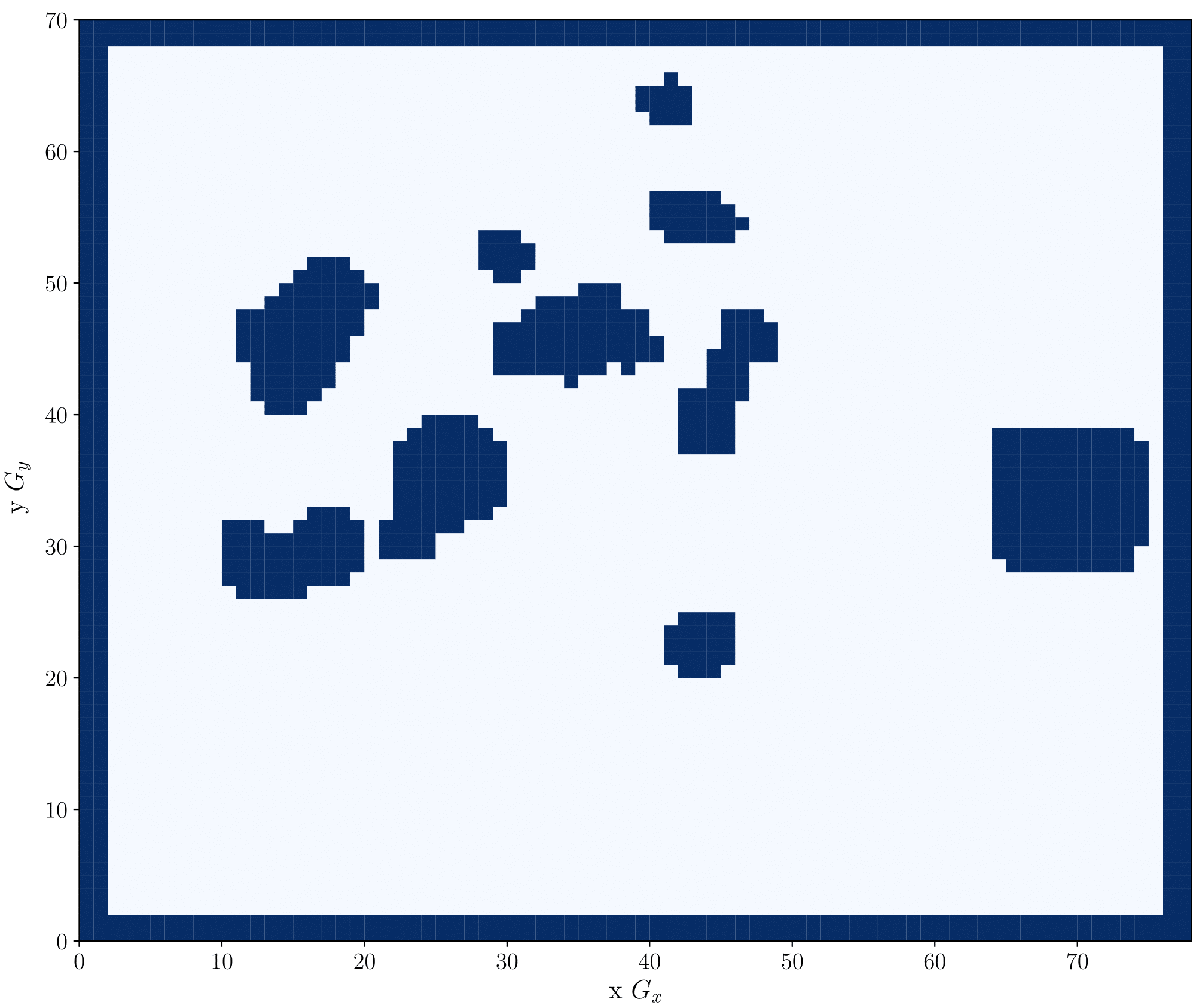
Fig 1: No-fly zones in Hong Kong airspace in geodetic coordinates (left) and corresponding obstacle map on the grid generated using Eq. (4) (right)
3. Initial Departure Phase Planning
The flight trajectory of the initial departure phase is constrained by the runway angle and the first direct-to-fix type leg direction. For example, HKIA has two parallel runways, as shown on the left-hand side of Fig 2. In the figure, "25L/R" indicates left and right runways with 250° heading angle, and "07L/R" indicates left and right runways with 70° heading angle. Six initial departure paths are designated by Hong Kong CAD accounting for the spatial separation near the airport, from one of two runways to one of three fixed points as shown on the right-hand side of Fig 2.** Each SID track in the Hong Kong AIP includes one of these six flight paths; hence we treat it as an initial departure path constraint in this study.
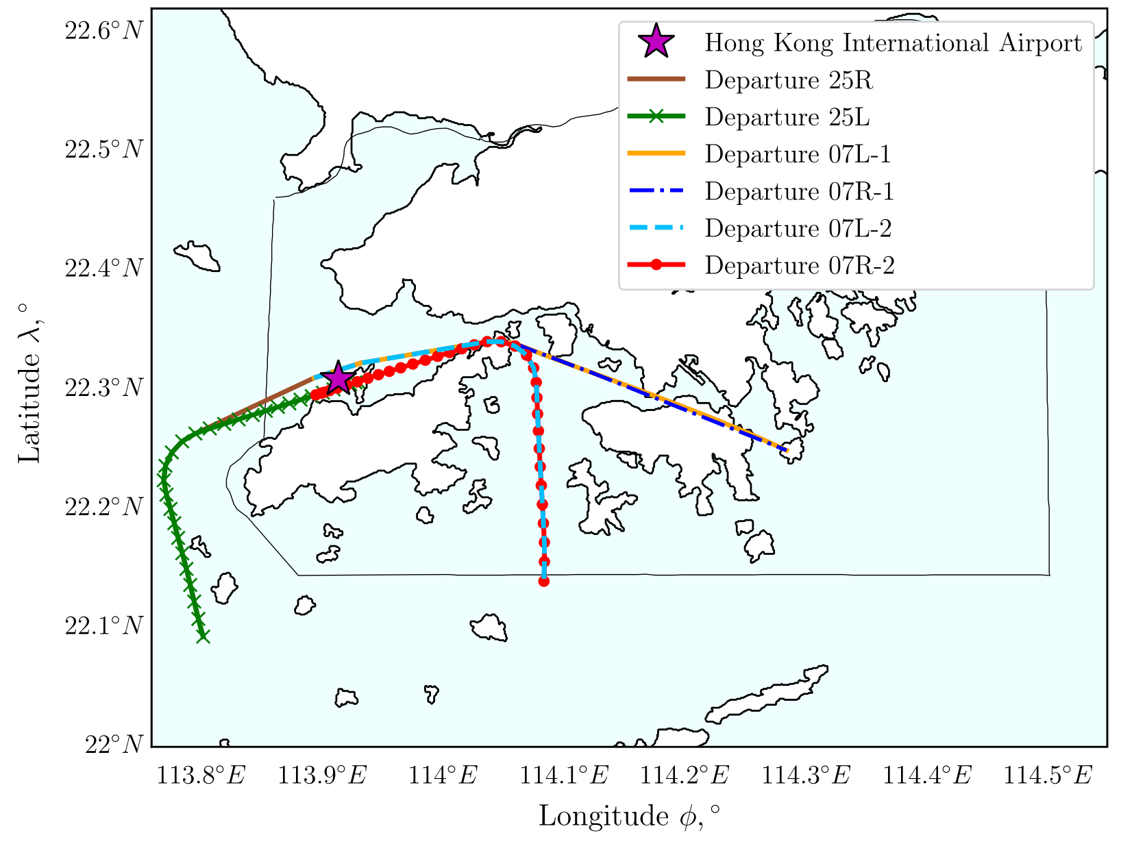
Fig 2: Runway configuration of HKIA (left) and the six initial departure paths from HKIA runways to the end of direct-to-fix legs (right)
Dubins path method is implemented to model the initial departure path constraint. This path is the shortest curve connecting two points in space, in which the curvature of the path is constrained by steering/heading angles [37]. It can enforce tangency constraints on the orientation at the start and endpoints [38]. These features provide a convenient framework for generating a path parallel to the runway and toward the direction of direct-to-fix legs. Six example configurations of Dubins paths are shown in Fig 3. These paths are compositions of R-L-S curves, where R is a right turn, L is a left turn, and S is a straight line. The Dubins path method first generates six paths with given start  and end
  points and corresponding heading angles
  . This procedure corresponds to the solution of the system of differential equations shown in Eq. (5), and the path distance D is evaluated by Eq. (6) from the solution
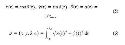
where the dot notation (e.g.,  ) denotes time derivatives,
  is the heading rate bounded by a maximum heading radius
  , and
, and  is the heading angle, which is the angle between the unit tangent vector
  and the
  axis. The path with the minimum distance is selected.
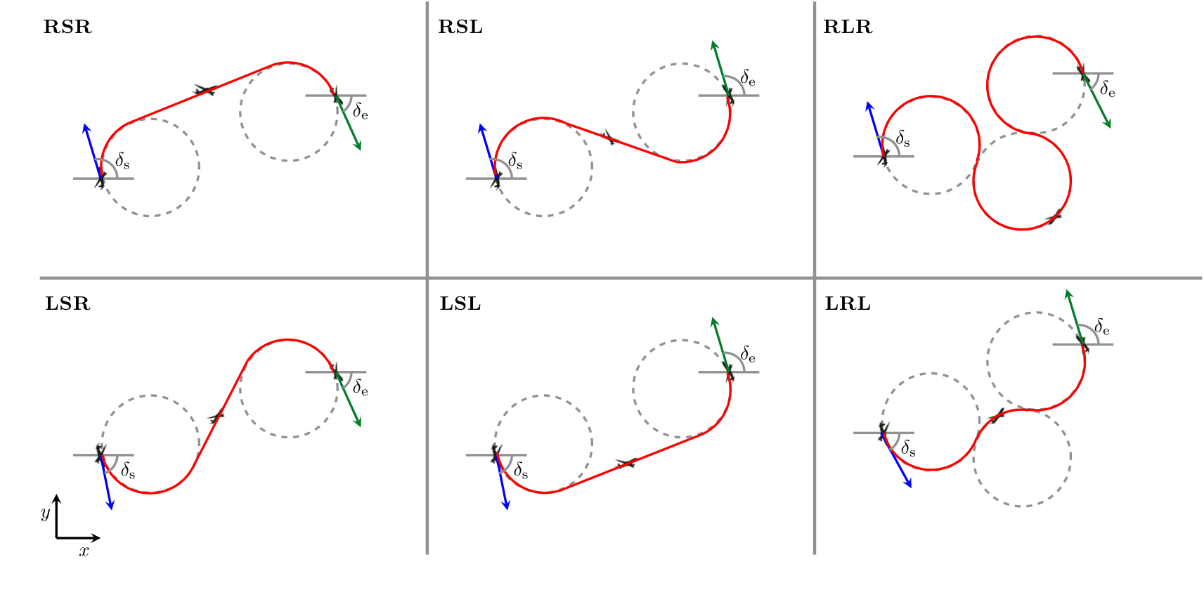
Fig 3: Six configurations of Dubins path with start and end heading angle constraints (), where R, L, and S denote right turn, left turn, and straight line respectively
4. Subsequent Departure Phase Planning with Population-Aware Constraints
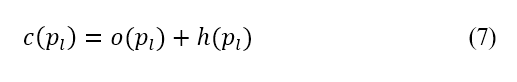
For a flight path plan that considers noise impact, perceived noise reduction over populated regions should be prioritised. These regions differ from no-fly zones where no flights are allowed, as the aircraft is still permitted to fly over populated regions, but it is not the preferred option. To reflect this characteristic in path planning, we incorporate a potential field formulation in the A* algorithm. The A* algorithm finds the shortest path on a grid with the lowest cost by evaluating the distance travelled on the grid while the object moves from the starting point to the target [39]. The cost function of the A* algorithm  can be expressed as
where  is the next node on the grid along the path,
  is the cost of the path from the starting node
  to
to  , and
, and 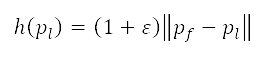 is a heuristic cost that indicates the cost of the least expensive path from to the target
  with tie-breaking factor
  . In our approach, the artificial potential field is formulated only with repulsive forces without modelling attractive forces for the target, in contrast to the standard potential field approach. We call this the population-aware A* method. The repulsive potential is used as a weighting factor for the cost function in Eq. (7). The modified cost function
  to consider the repulsive potential and shortest travel distance is given by
where the term  is the normalised repulsive potential, which is calculated based on local population data and is described below. To obtain the population data, we use the administrative unit centre locations with population estimates from the NASA Socioeconomic Data and Applications Center.†† Population data are specified in terms of the centre location
  , area
  , and population estimate
  for sublevel administrative units. The sources of the repulsive potential are placed at the corresponding centre location of each sublevel administrative unit, which is represented as a circle. Consider
  such sources, then the potential field is determined by the sum of the influences of these sources at every point on the grid
  . The repulsive potential
  at measuring position
  is dependent on sources located at
  with strength
  given by the population estimate at
  , as described previously. The potential at induced by a single source located at is also dependent on the distance to the source
  , and its radius corresponding to the effective area A, which is computed as
  by the circular representation of the sublevel administrative unit. The distance to the source is computed by Haversine's formula [36]. We note that is in geodetic coordinates. The transformation between
  on the grid and
  is given by
  [see Eq. (3)] for consistent measures of distance. The potential field
  accounting for all of these terms can be expressed as
As the source is not treated as an obstacle, the path of the aircraft can still pass through its region. In other words, the magnitude of the repulsive potential should not cause the cost function used in path planning to approach zero or infinity in the limit. This constraint is imposed by normalising the repulsive potential to the range  . This normalisation is calculated by
where  and
and  are the maximum and minimum repulsive potential values of the entire potential field respectively.
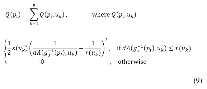
Following the previous examples pertaining to Hong Kong airspace, the proposed potential field is computed using Hong Kong's population data. The population distribution is shown on the left-hand side of Fig 4. The potential field computed based on the population is shown on the right-hand side of Fig 4. The repulsive potential shown on the right is conceptually a superposition of the influences from the population densities at the respective sources, which is computed based on the population distribution shown on the left.
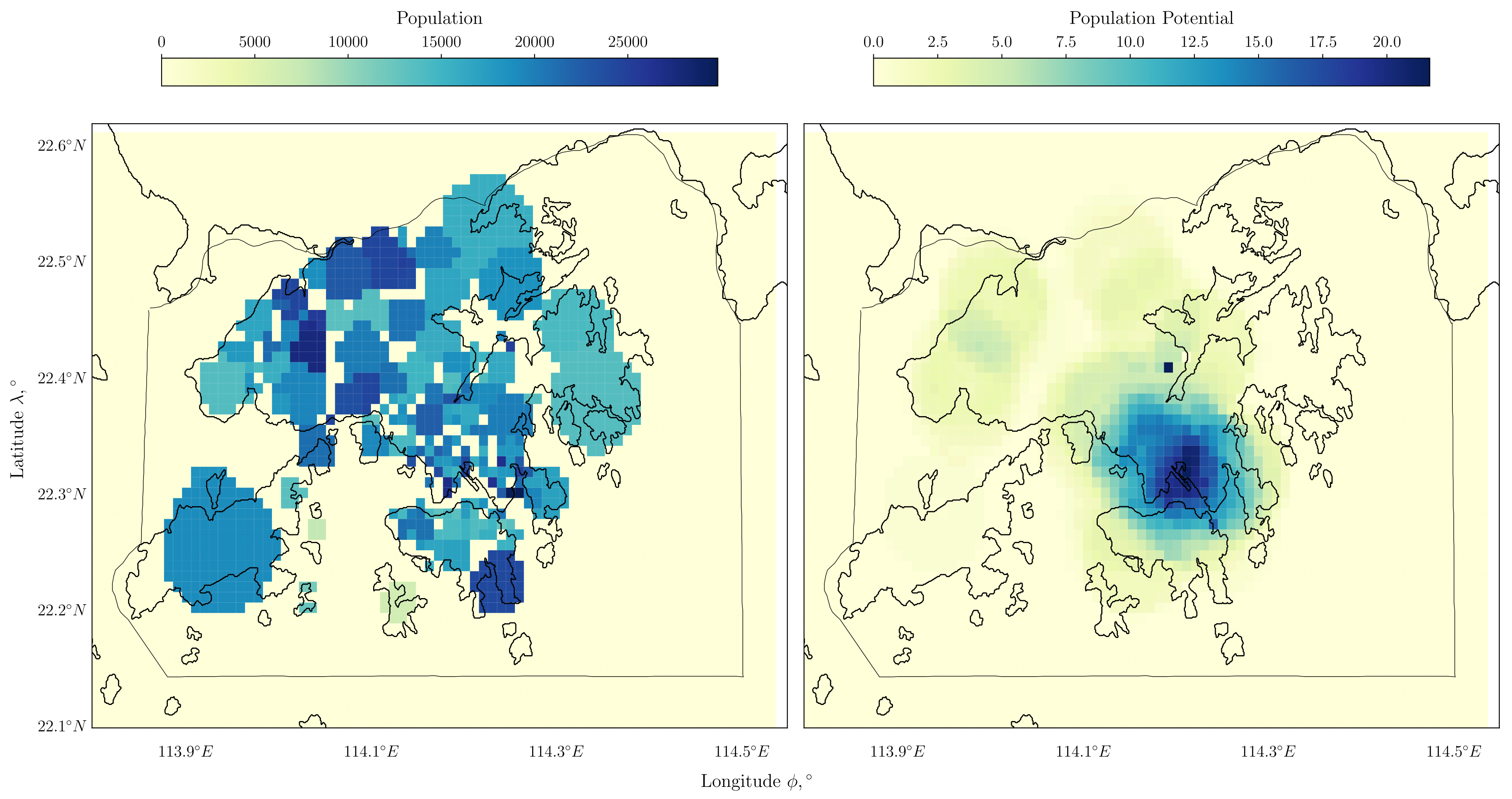
Fig 4: Population distribution of Hong Kong (left) and corresponding potential field representation (right) generated using Eq. (9)
5. Subsequent Departure Phase Planning with Population-Aware and Steering Constraints
The population-aware A* algorithm described in Sec. II.A.4 finds the path minimising the cost function at the current node in Eq. (8) and then searches for the next node by testing movements in eight directions, as shown in the left-hand side of Fig 5. These moving directions are constrained by the geometric configuration of the grid nodes, which can result in an unphysical path. To address this issue, a refined search direction incorporating a concept from sampling-based path planning methods is defined in the developed method; an example is depicted in the right-hand side of Fig 5.
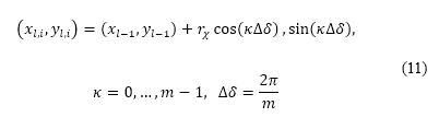
Let  , be the points corresponding to the current and next nodes of the path in Cartesian coordinates. To improve flexibility of the path, sample points are generated around
  at every angular interval
  on the perimeter of concentric circles with different radii
  . The right-hand side of Fig 5 illustrates this approach with
  rad and
  . The positions of the points generated for the samples in Cartesian coordinates
  , are computed by
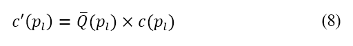
We also introduce a steering penalty to limit the changes in path angles, which takes into account the lateral manoeuvrability of an aircraft. This steering penalty via sampling is incorporated into the population aware A* method. We call this refinement the population-aware A* with steering constraints method. The refined cost function  is expressed as
where  is the cost function previously presented in Eq. (7), and the extended normalised potential
  and the steering penalty
  are described next. We extend the domain of , i.e., the normalised repulsive potential defined on presented in Eq. (10), to the domain by bilinear interpolation of the normalised potential computed on the four points adjacent to node
  in . We denote this extension as , which is used to compute the cost function Eq. (12).
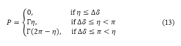
The steering penalty at the point to avoid steep path angle changes is applied only if the difference in angles between the previous path and the next path η is larger than the specified angle interval , which is used as the interval of the circular search direction. The penalty weight  is adjusted depending on the distance from the start node to the target node. The penalty increases as the difference between the previous and next path angles increases, expressed as
To an extent, this penalty acts as an inertial force when considering the manoeuvrability of an aircraft. The point with minimum cost evaluated by Eq. (12) is chosen as the next node on the path among the sample points, and the process is repeated until the aircraft reaches its target.
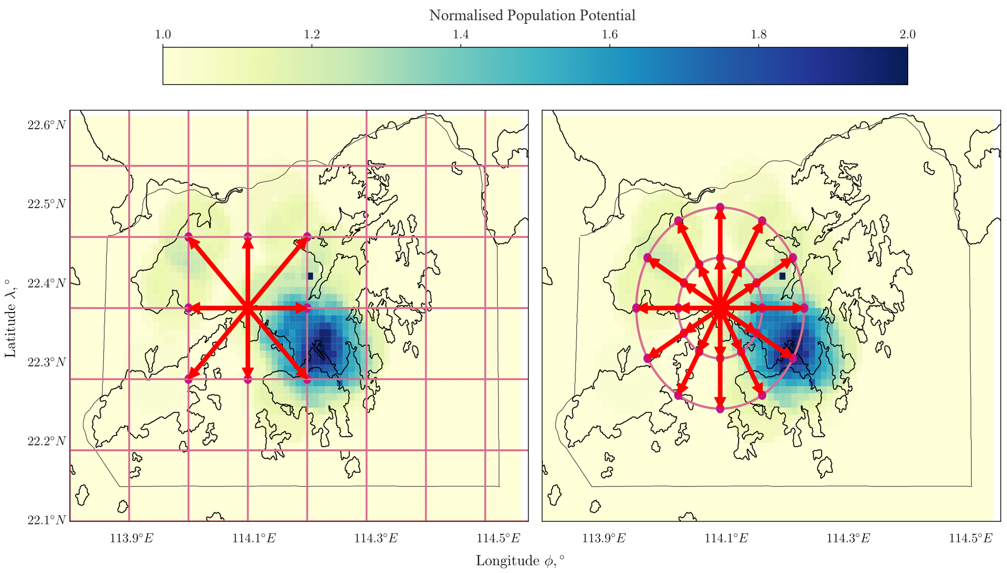
Fig 5: Eight possible moving directions (not to scale) of the A* algorithm and population-aware A* method on the grid (left) and 24 possible moving directions of population-aware A* with steering constraints method (right)
B. Altitude Path Planning
The surface path planning methodology described in Sec. II.A determines the shortest surface path to the compulsory ATS reporting point from the departure airport considering no-fly zones, runway angles, spatial separation of aircraft near the airport, populated regions, and steering constraints. Our developed altitude path planning methodology manifests a complete three-dimensional path along the generated surface path by evaluating the fuel consumption and the accumulated perceived noise level along the flight trajectory. In Sec. II.B.1, we present an optimisation formulation that minimises fuel consumption and noise levels along this trajectory. Section II.B.2 describes a longitudinal flight simulation methodology that generates a flight path to the target while computing the corresponding fuel consumption. Section II.B.3 describes the method for evaluating the noise level along this flight path.
1. Optimisation Problem Formulation
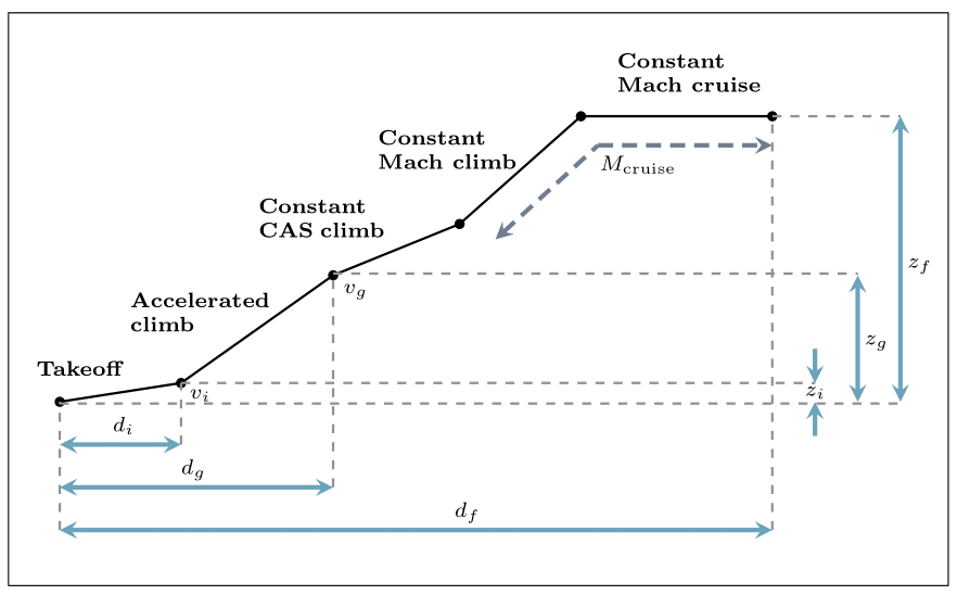
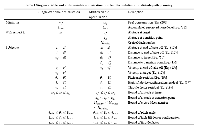
Two formulations for the altitude path, single-variable and multi-variable optimisation, are proposed in this study, depending on whether the upper bound of the altitude along a path changes. We describe these two formulations by referring to Fig 6. As an example, suppose that the aircraft departs from HKIA, marked as the pink star in Fig 6a. It must pass one of the compulsory ATS reporting points, marked as black triangles, which is a target of our path planning method. The upper bound of the flight level in the dark blue region is constrained to 25,000 feet by AIP regulation. The single-variable formulation is used for path planning from HKIA to the reporting points within this region, such as BEKOL, TAMOT, and SIERA, indicated by blue text in Fig 6a. The multivariable optimisation problem is formulated for path planning from HKIA to points placed on the region with flight level "Surface to unlimited" (terminology used in AIP) whose upper altitude limit is unbounded, indicated by the grey region in Fig 6a. The details of the two formulations are summarised in Table 1 and described below.
We assume that the altitude path generated by single-variable optimisation is composed of two flight segments: take-off and accelerated climb, as presented in Fig 6b. The take-off and accelerated climb segments in the figure correspond to the initial and subsequent departure phases of the surface path, respectively. Flight simulations to determine the path (elaborated in Sec. II.B.2) are performed by implicitly determining the pitch angle  , high-lift device configuration
  , and throttle factor
  at the
  time step of the simulation, and explicitly imposing boundary conditions in terms of distance
  , altitude
  , and velocity
  for each segment. The distances to the ends of take-off and accelerated climb segments
  are obtained from the initial and subsequent departures of the surface path. The altitude
  and velocity
  at the end of take-off are fixed depending on the aircraft type and loading conditions. The target altitude at the end of the accelerated climb
  is a design variable of the single-variable optimisation, as presented in the second column of Table 1. The changes in the target altitude lead to changes in the vertical flight profile related to operational conditions such as engine power and aircraft speed. These conditions further contribute to the changes in accumulated perceived noise level
  and mass of fuel consumed
  . Hence, we minimise fuel consumption and accumulated perceived noise with respect to the target altitude, as shown in Table 1. A flight path that transitions between varying upper flight level bounds is modelled by multivariable optimisation, as presented in the third column of Table 1. This path is assumed to have five flight segments as illustrated in Fig 6c: take-off, accelerated climb, constant calibrated airspeed (CAS) climb, and constant Mach number climb and cruise. The take-off segment in multivariable optimisation also corresponds to the initial departure phase of the surface path, and the remaining segments correspond to the subsequent departure phase of the surface path. The cruise Mach number
  and altitude at the transition point
  are treated as design variables in addition to the altitude at the target point. This transition point on the path is located on the boundary between the blue and grey regions in Fig 6a, where the upper limit of flight level transitions from 25,000 feet to unlimited. We set this point at the end of the accelerated climb segment, and additional boundary conditions (regarding altitude, distance, and velocity) at the point are also considered. The altitude of the point is one of the design variables as previously described. The distance to point
  is determined from AIP. As subsequent flight segments after accelerated climb are of constant speed type (constant CAS or Mach number), and the cruise Mach number is one of the design variables, the speed
  at the transition point is determined by the cruise Mach number and altitude at the transition point by the following equation:
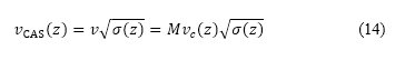
where is true airspeed,  is density ratio, and
  is the speed of sound. We assume that the equivalent airspeed is equal to the calibrated airspeed
  . In Table 1, symbols with an asterisk denote given boundary conditions explained above for the flight simulation methodology. Lower and upper bounds of the flight altitude at compulsory ATS reporting points
  and at the transition point
  are provided in the AIP. The variation of cruise Mach number is limited to the range between the lower and upper Mach numbers
  based on the aircraft type and its operating conditions. The high-lift device configuration and throttle factor are bounded in the interval
  , and the pitch angle is bounded by the appropriate operating conditions for take-off, climb, and cruise. The method used to solve these single-variable and multivariable multi-objective optimisation problems is based on the non-dominated sorting genetic algorithm II (NSGA-II), which is a fast sorting and elite multi-objective genetic algorithm [40].
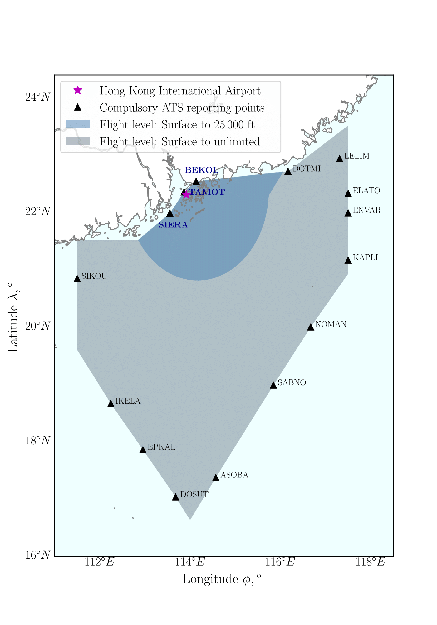 a) Flight level restrictions in Hong Kong airspace
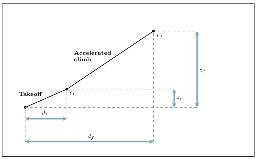 b) Flight segments for single-variable optimisation (not to scale)
 c) Flight segments for multivariable optimisation (not to scale)
Fig 6: Map of flight level restrictions a) influencing the selection of single-variable and multivariable optimisation and the combination of flight segments to model a departure path for single-variable optimisation b) and multivariable optimisation c)
It creates  numbers of population with design variables, combining parents and offspring generated by crossover and mutation. The objectives are then evaluated for this population and sorted in a list by their rank and crowding distances in an increasing order. The rank represents the order of layers of the solutions based on the dominance. For example, with design variable values
  and
and  , has higher rank than when dominates , defined as
  in the optimisation problem of minimising two objectives
  and
and  with respect to . The crowding distance represents the density of the solution. If both solutions belong to the same rank, the solution that is located in a less dense region is assigned a higher priority. The first half of the sorted list is evolved to the offspring, constituting the population for the next generation.
Two features to improve the computational efficiency of the optimisation process are implemented in this study. First, unlike a conventional NSGA-II exploring a continuous domain, NSGA-II with integer programming is used to perform discrete optimisation. Although our design variables correspond to continuous physical quantities, a discretisation considering their practical meaning promotes efficient exploration of the design space. For instance, we can evaluate noise and fuel consumption with target cruise altitude 11,000.0 and 11,000.1 m and mathematically conclude that one of the conditions is better, which seems practically meaningless in the context of air transportation routes. Instead, we evaluate the objective functions with target altitude 11,000 and 11,100 m in the same computation time to find the broad trends of the objective function variations. To consider design variables with specified intervals, we use a real-coded genetic algorithm with random integer sampling in NSGA-II, instead of implementing a binary-coded genetic algorithm commonly used in discrete optimisation. The values of the design variables generated are integers, within lower and upper bounds 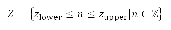 . The optimisation parameters, such as population size and the number of generations, are set such that at least 20% of the design space is covered owing to the finite number of design variable values. Second, the solution evaluation of repeated design variables is prevented by the technique called memoization in dynamic programming [41]. It speeds up the optimisation process by storing the results of fuel consumption and accumulated noise evaluation, which are obtained by running time-consuming flight simulations, and returning the cached result when the same value for the design variable occurs again.
2. Fuel Consumption Estimation
We evaluate the fuel consumption along the altitude path by employing a data-enhanced flight simulation method developed by the authors [42]. The method enables longitudinal flight path generation and fuel consumption estimation with information available from preliminary aircraft design stages and historical flight data for various aircraft types. The flight simulation procedure has previously been validated against actual flight data for short-, medium-, and long-haul flights with approximate errors less than 7%. The flight simulation solves the governing equations of motion presented in Eq. (15) for the aircraft position and velocity as an initial-value problem with fixed boundary conditions:
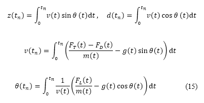
The equations are discretised using finite differences and are integrated forward in time  . Distance , velocity and altitude to the end of initial and subsequent departure phases are specified as boundary conditions from the surface path planning and optimisation settings. The initial values of the mass
  , velocity, distance, altitudes, and pitch angle are also specified. The values of thrust
  , lift
  , and drag
  forces, and the gravitational acceleration
  are then computed with these initial values and used to find velocity, pitch angle, distance, and altitudes at the next time step. When the computed velocity, distance, and altitudes meet the requirements at the endpoint of subsequent departure phases, the simulation is terminated, which implies that the total flight time
  depends on the boundary conditions. Specifically, the thrust model used in this study accounts for changes in altitude and speed through the density ratio , Mach number
  , and throttle factor as shown
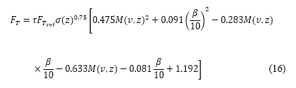
where  is the reference thrust of the aircraft's engines, and
  is their bypass ratio. Both parameters depend on the engine type and are assumed as constants. The Mach number and density ratio are functions of speed and altitude:
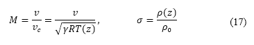
where is the speed of sound, which is a function of heat capacity ratio of air  , gas constant
  , and atmospheric temperature . The air density, pressure, and temperature are determined by the International Standard Atmosphere model [43]. The variation of gravitational acceleration with altitude is calculated via a spherical approximation of Earth's shape.
The aerodynamic forces (lift and drag ) are computed with air density, velocity, wing area  lift coefficient
  and drag coefficient
  as expressed:
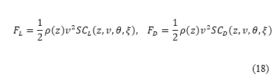
where represents modifications for high-lift device configurations. The lift and drag forces implicitly account for altitude, velocity, pitch angle, and high-lift device configurations. In particular, the lift coefficient is determined by the Polhamus formula [44] and Dubs's model [45] as an explicit function of the angle of attack (same as pitch angle in this study), Mach number (which is a function of altitude and velocity), high-lift device configurations, and other fixed aircraft information, such as the wing aspect ratio, fuselage width, sweep angle, and wing span. The drag coefficient is determined by an empirical drag build-up method of profile drag, induced drag, and wave drag as an explicit function of the lift coefficient, Mach number, and also other aircraft information, such as the wing reference area, wing wetted area, wing span, mean chord length, fuselage width, fuselage tail cone length, nacelle length, and wing aspect ratio [46]. The values of pitch angle, high-lift device configuration, and throttle factor at each time step of the simulation are determined by solving the following optimisation subproblem:
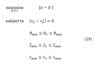
where variable  in the objective function
  depends on the type of flight segment: is the x-directional acceleration for the take-off and accelerated climb segments, calibrated airspeed for the constant CAS climb segment, and Mach number for the constant Mach climb and cruise segments, and
  is the corresponding required value for each of the properties, which is implicitly determined from the boundary conditions. Hence, minimising the absolute difference between and forces the properties to be maintained as constants during the corresponding flight segment. Similarly, the vertical speed
  is also a constant for each segment, and the target vertical speed
  is determined by the data analysis presented in [42]. Each design variable is bounded by its respective minimum and maximum, denoted by subscripts "min" and "max" in the variable bounds, which vary with the flight segment type. High-lift device configurations are only considered during take-off and accelerated segments, in which flaps and slats are deployed.
The fuel consumption is computed from the discretised form of
which depends on the thrust, gravitational acceleration, and specific fuel consumption  at each time step of the simulation. The specific fuel consumption is determined using a surrogate model built from an engine dataset via the open-source library Surrogate Modelling Toolbox (SMT) [47], depending on the altitude, velocity, and throttle factor.
3. Accumulated Perceived Noise Level Estimation
The accumulated perceived noise level is evaluated using the Noise-Power-Distance (NPD) table in the Aircraft Noise and Performance (ANP) database‡‡ from Eurocontrol. The ANP/NPD database is an online data resource for estimating the noise impact induced by an aircraft. It presents a wide choice of aircraft types, operations, and acoustic models accompanying the ECAC Doc. 29 and ICAO Doc. 9911 guidance documents [48,49].
We use an A-weighted sound exposure level model from the ANP database for the perceived noise level, which represents the total sound energy integrated over a second and is tailored to the sensitivity of the human ear. It depends on the aircraft type, engine thrust, operating modes (such as departure or approach), and the distance from the aircraft to the observer [50]. The aircraft selected for the path planning fixes the type as constant. The operating mode is also a constant as we only consider departure path planning in this study. Engine thrust and distance are determined by the flight simulation described in Sec. II.B.2. An observer is assumed to be located on the ground at sea level below the aircraft in our study; hence the distance to the observer equals the altitude . The accumulated perceived noise level along an altitude path is obtained from the following expression:
where  is the time step used for the flight simulation, explained in Sec. II.B.2, and
  is the A-weighted sound exposure level at the
  time step. As the accumulated sound exposure level strongly depends on the maximum due to the logarithmic sum, we only consider the sound exposure level of the climb segments during the optimisation process to clearly observe the effects of changing the altitude path to the accumulated noise level.
III. Results and Discussion
This section presents surface path planning results and an optimal set of altitude paths along two flight routes, Hong Kong to London and Hong Kong to Taipei, as case studies. The flight simulation parameters are based on a Boeing 777-300ER with GE90-115B engines. The developed path planning and optimisation procedures presented in Sec. II are implemented for flights departing from HKIA (22°18'32.0''N, 113°54'52.0''E) passing compulsory ATS reporting points, i.e., BEKOL (22°32'36.0''N, 114°08'00.0''E) for aircraft heading to London Heathrow Airport and ENVAR (21°59'29.8''N, 117°30'00.0''E) for aircraft heading to Taiwan Taoyuan International Airport.
A. Surface Path Planning
We present the optimised surface paths generated using the methodology in Sec. II.A for the Hong Kong–London route (Fig 7) and the Hong Kong–Taipei route (Fig 8). The visualisations presented in these figures will be described before we discuss the specific results for each route.
In the figures, the location marked by a star corresponds to HKIA, which is the starting point of the path planning. The site marked by a black triangle is the compulsory ATS reporting point, which is the target point of path planning. The areas marked in red are the obstacles mentioned in Sec. II.A.2, which the aircraft cannot pass through. The black lines represent the boundary of the country and its coastlines. The superimposed colour indicates the strength of the normalised population potential field. The dark blue areas have a high population density and are not favoured to be flown over by the aircraft as mentioned in Sec. II.A.4. The corresponding SID track is depicted as a bold grey line, linking SID guide points marked using circles with black outlines. Nine flight paths generated by Quick Access Recorder (QAR) data of Boeing 777-300ER flights are depicted as purple lines. The QAR records detailed information of aircraft operations during flight, such as position, attitude angles, airspeed, weight, etc. In this study, the longitude, latitude, pressure altitude, thrust, and weight information from QAR data are used for comparison and validation. The path planning results are denoted by four colours. Dubins path, depicted in orange, is the path generated for the initial departure phase mentioned in Sec. II.A.3, and is a common path of the three subsequent departure paths. These three path plans, starting from the end of Dubins path to the target, are presented under the names of A*, population-aware A*, and population-aware A* with steering constraints. From here onward, we will refer to these three methods as A*, PA*, and PA*S respectively for brevity and readability.
The A* path, depicted in blue, is the result of applying the A* algorithm considering only obstacle constraints mentioned in Sec. II.A.2. The cost function expressed in Eq. (7) is used to generate this path. The PA* path, depicted in green, is the result of applying the populated region constraints mentioned in Sec. II.A.4 along with obstacle constraints. The cost function expressed in Eq. (8) is used to generate this path. The PA*S path, depicted in magenta, is the result of applying steering penalty considerations in addition to obstacles and populated region constraints. The cost function expressed in Eq. (12) is used to generate this path. The PA*S path represents the developed surface path planning methodology in this paper, which finds the shortest path avoiding obstacles and highly populated regions while accounting for aircraft manoeuvrability with a steering penalty.
1. Hong Kong to London
The surface path plans for the aircraft departing from HKIA and heading to London Heathrow Airport are depicted in Fig 7. This route passes a compulsory ATS reporting point named BEKOL, which is designated by Hong Kong AIS. Departure 07R-1 shown in Fig 2 is chosen for the initial departure path in this simulation based on the location of BEKOL. This selection is also consistent with our observations of most QAR flight path data corresponding to aircraft that fly to BEKOL. The SID track, which uses departure 07R-1 to BEKOL is presented as a line connecting HKIA–ROVER–TUNG LUNG–ATENA–BEKOL. The initial departure phase, which starts from HKIA, is set to end at a point on the ROVER and TUNG LUNG line. This point is selected close to a densely populated region to observe the variations of the paths generated by the different planning methods. The subsequent departure phase corresponds to the flight segment from this point to BEKOL. It is found that the generated Dubins path satisfies the initial departure path constraint and avoids obstacles around the airport. Subsequently, the A* algorithm without considering the population creates the shortest path that traverses inland Hong Kong over a highly populated region. In contrast, the PA* and PA*S methods generate routes that avoid this area with a high normalised population potential field. As PA*S, which operates on Cartesian coordinates, has a higher degree of freedom in path planning than PA*, which operates only on grid points, less abrupt changes in heading direction are observed when the steering constraints are included.
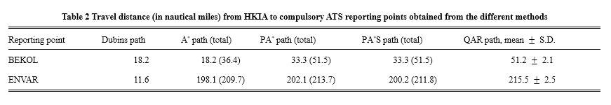
PA*S with Dubins path is the most similar to the SID track and the QAR paths among the three results. Particularly, the initial departure path is almost identical to the SID track and QAR paths. Dubins path from HKIA to ROVER, which is constrained by runway angles, is almost parallel to the SID track and QAR paths. The QAR paths deviate from Dubins path and the SID track between ROVER and TUNG LUNG, flying over populated regions and eventually passing over the eastern outskirts of Hong Kong at ATENA toward BEKOL. The PA* path matches the SID track more closely in comparison to the QAR paths while turning nearer the SID guide point TUNG LUNG toward ATENA, showing that the developed method can be used to support SID planning. In addition to this similarity, flyability can be determined by the initial and final path angles of the PA*S path. The initial path angle, around TUNG LUNG, follows from the angle at the end of the initial departure phase, and so the path steadily moves toward the target. The final path angle at the end of the subsequent departure phase, near BEKOL, is similar to those of QAR paths, which represents a physically flyable route as validation. Table 2 presents path lengths computed from each path planning method. The first column represents the distance computed in the initial departure phase from Dubins path. The following three columns represent the distances computed in the subsequent departure phase using the path planning methods presented in this paper. The path length written inside parentheses "(total)" of these columns refers to the total distance travelled during the initial and subsequent departure phases. This is computed by adding the corresponding distance obtained from Dubins path for the route to the subsequent departure path distance obtained from each method. The last column shows the average and standard deviation (S.D.) of the nine QAR path lengths shown in Fig 7. To assess our results, we compare the total lengths for A*, PA*, and PA*S paths with the average QAR path length. In this case, the average QAR path length (51.2 nautical miles) is 0.3 nautical miles shorter than the total PA*S path length (51.5 nautical miles). Note, however, that the QAR paths traverse areas with high population potential, instead of those with low population potential. As such, the PA*S path constitutes an improved solution that avoids populated regions, which potentially contributes to lower noise impact, without any significant increase in travel distance.
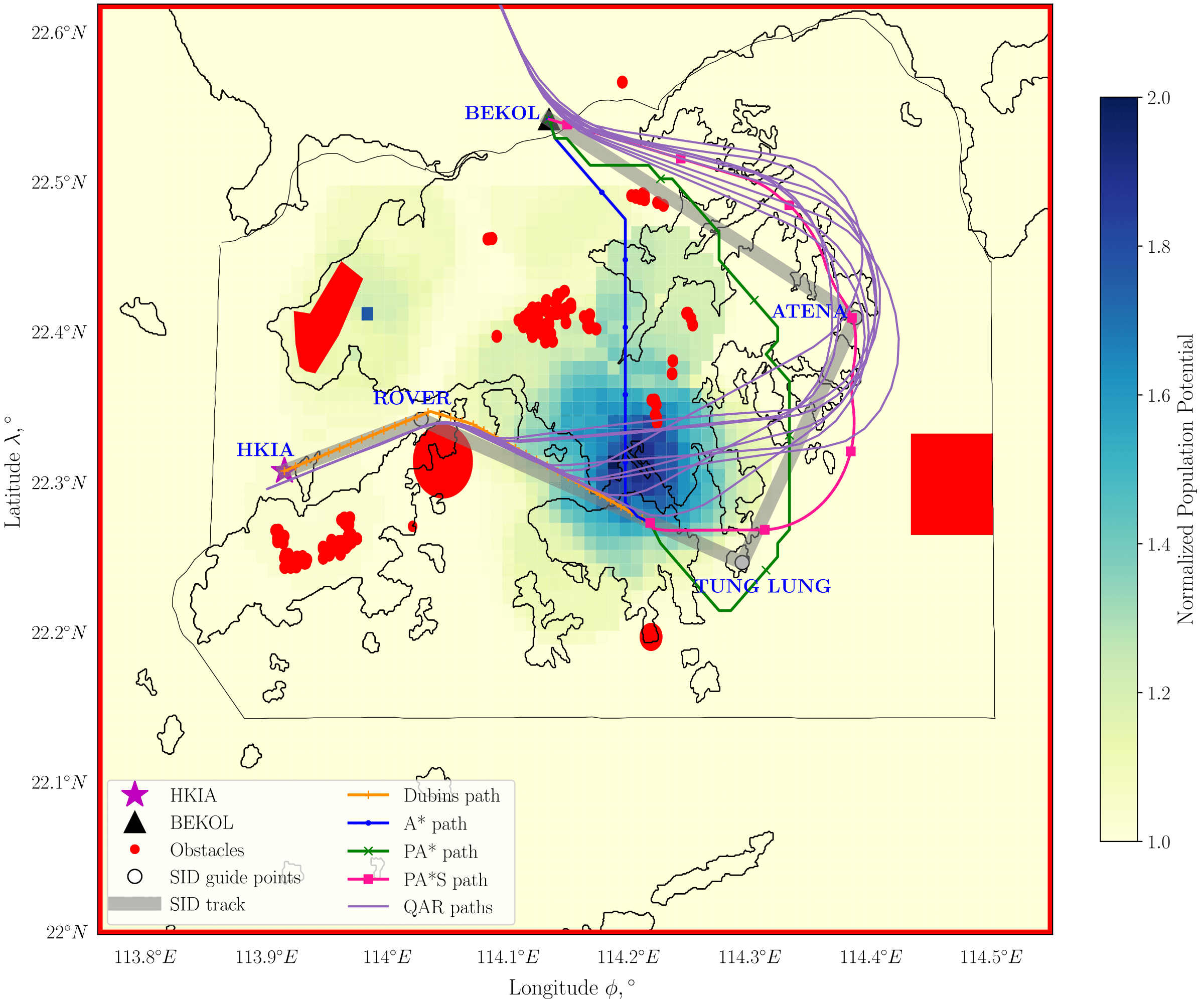
Fig 7: Surface paths from HKIA to BEKOL (Hong Kong–London route) with obstacles and the normalised population potential over Hong Kong airspace
2. Hong Kong to Taipei
Surface path planning for an aircraft departing from HKIA and heading to Taiwan Taoyuan International Airport is depicted in Fig 8. This route passes a compulsory ATS reporting point named ENVAR, which is also designed by Hong Kong AIS. The target point is located far southeast of Hong Kong, so the figure on the left-hand side of Fig 8 is enlarged, centring on the Hong Kong Territory, and presented on the right-hand side. The SID track to ENVAR is similarly depicted as a grey line, connecting HKIA-ROVER-ROBBE-RAMEN-OCEAN-ENVAR. The initial departure phase is set for the aircraft to depart from HKIA to ROBBE, to provide flexibility for the path planning method to move along either Departure 07R-1 or 07R-2 (referring to Fig 2). The subsequent departure phase is set to move from ROBBE to ENVAR. In the close-up figure on the right-hand side, Dubins path is almost parallel with the SID track and QAR paths, satisfying the initial departure path constraint. Subsequently, the A* algorithm generates a path similar to that of the Departure 07R-1 track, passing through areas with high population potential. In contrast, the PA* and PA*S methods generate routes similar to the Departure 07R-2 track, which tends to avoid areas with high population potential.
The A* path, which is the shortest, still passes through the region with high population potential following the Departure 07R-1 track. Approximately 70% of the QAR paths also pass through this region, which can negatively affect the noise impact. The remaining QAR paths, which follow the Departure 07R-2 track, are quite similar to the PA*S path and the SID track. The PA*S path deviates from the SID track between RAMEN and OCEAN, as shown on the left-hand side of the figure. This deviation particularly contributes to the shorter path length, as shown in Table 2. The average travel distance of the QAR path is about three nautical miles longer than those of the PA*S paths for this route. This difference is mostly caused by large turns around OCEAN, as can be seen in Fig. 8. We observe that some QAR paths do not pass OCEAN, resulting in paths similar to that of PA*S. This observation shows that the generated PA*S path is flyable. Although our method generates a shorter route than most QAR paths, it does not consider certain air transportation restrictions, such as the air traffic conditions involving multiple aircraft flying on similar routes. However, unlike PA*, PA*S maintains the flight direction at ROBBE, which is attributed to the steering constraints acting like an inertial force, and hence can also model current flight operations as shown in the QAR paths. Additionally, the sharp turns seen in A* and PA* paths, which are constrained to the grid points, are not observed in the PA*S path.
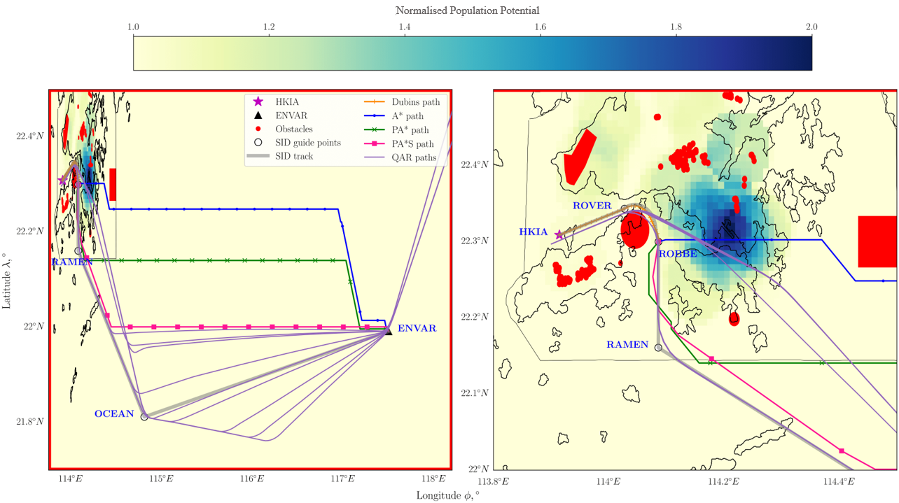
Fig 8: Surface paths from HKIA to ENVAR (Hong Kong–Taipei route) with obstacles and the normalised population potential over Hong Kong airspace
B. Altitude Path Planning
We present the altitude paths of the two scenarios shown in Sec. III.A by performing multi-objective optimisations for low-fuel consumption and low-noise impact. The paths from HKIA to BEKOL are obtained by performing single-variable optimisation, and the paths from HKIA to ENVAR are obtained by performing multivariable optimisation, following the formulations described in Sec. II.B. Unlike the surface path planning methodology, which yields a single shortest path, multiple altitude paths are obtained as a solution set of multi-objective optimisation. These are represented by the graphs shown on the left-hand side of Fig 9 and the top of Fig 10, in which the horizontal axis is the travel distance, and the vertical axis is the altitude. The feasible region of the optimisation and a Pareto front for low-fuel consumption and low-accumulated perceived noise level are presented on the right-hand side of Fig 9 and the bottom of Fig 10. The feasible region refers to all solutions evaluated by the modified NSGA-II algorithm during optimisation. This region is displayed with a colour map representing the altitude for single-variable optimisation in Fig 9, and in light blue for multivariable optimisation in Fig 10. Note that the same colour convention is also used to identify the corresponding altitudes of the optimisation solutions shown on the right-hand side of Fig 9. Among the feasible solutions, the nondominated solutions, viz., the Pareto front, are indicated by solid magenta lines and triangles. Similar to the surface path illustrations, the altitude variations of the QAR paths are displayed as dotted purple lines and purple stars. The purple stars on the left-hand side of Fig 9 and the top of Fig 10 depict the points closest to the corresponding compulsory ATS reporting point of the respective paths, and the ones on the right-hand side of Fig 9 denote the respective fuel consumption and noise levels for comparison with the solutions.
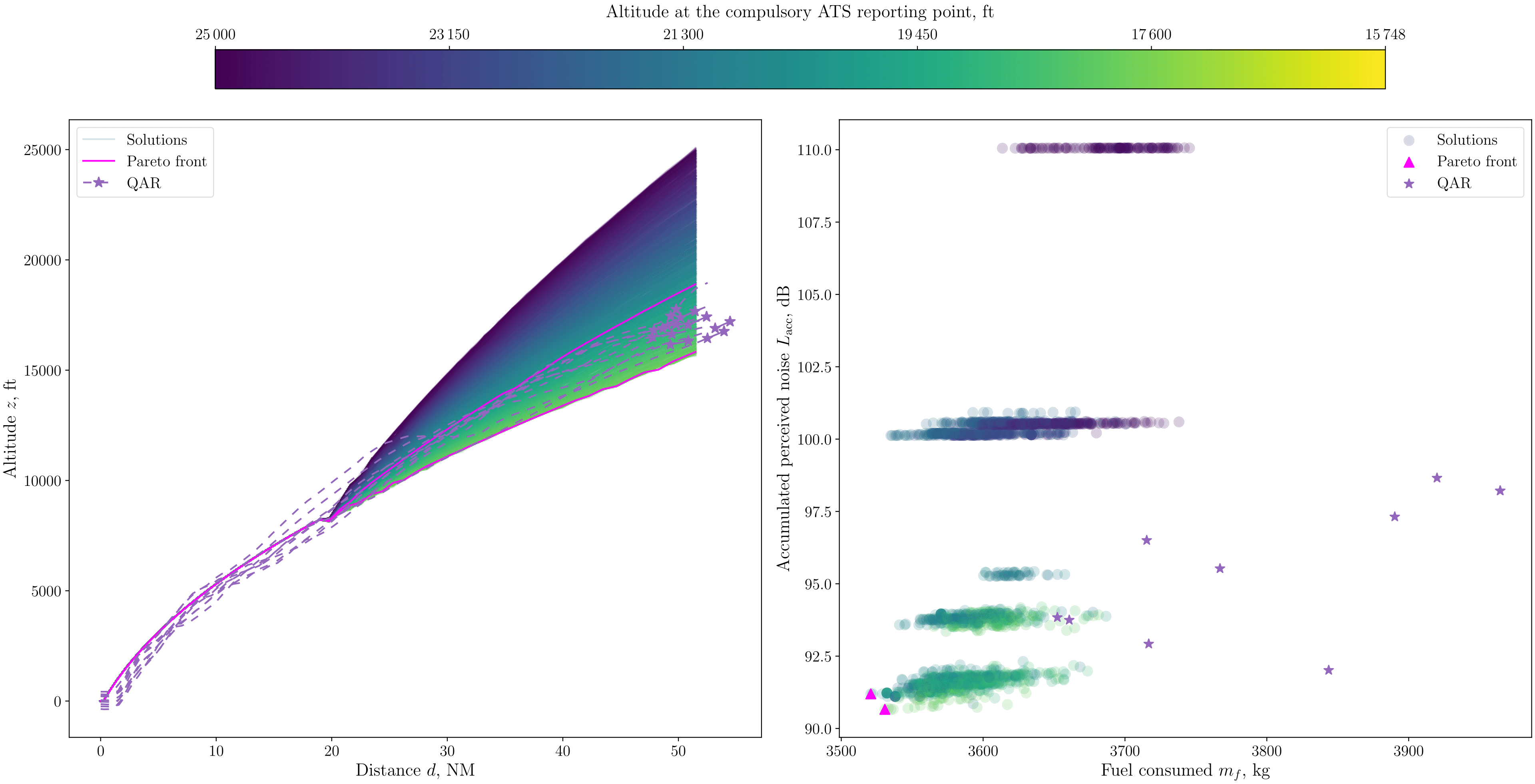
Fig 9: Feasible solutions of altitude path optimisations, their Pareto front, and QAR data from HKIA to BEKOL (left) and corresponding fuel consumption and accumulated perceived noise levels (right)
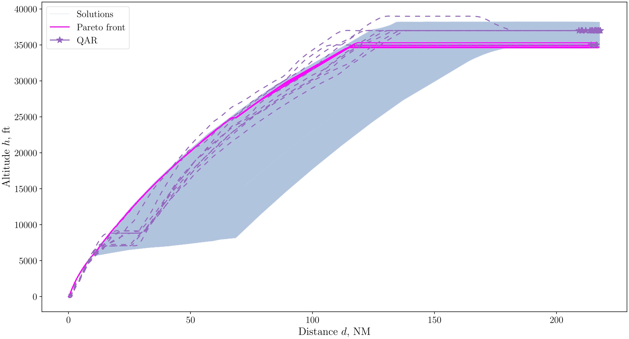
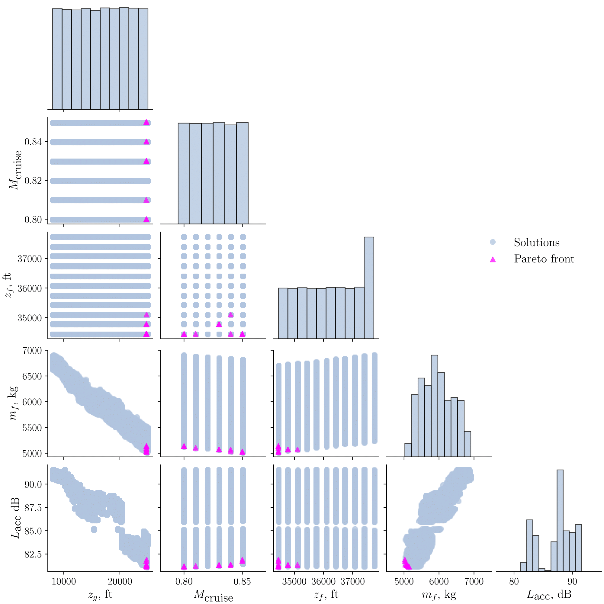
Fig 10: Feasible solutions of altitude path optimisations, their Pareto front, and QAR data from HKIA to ENVAR (top), and fuel consumption and accumulated perceived noise level with respect to three design variables, viz., target altitude, transition point altitude, and cruise Mach number (bottom)
The altitude paths consist of initial and subsequent departure paths similar to the surface paths. The initial departure path, which corresponds to the take-off segments shown in Figs 6b and 6c, is the path with only one magenta line on the left-hand side of Fig 9 and on the top of Fig 10. This corresponds to the Dubins path portion of the surface path plan. The travel distance of Dubins path, given in the second column of Table 2, is the total distance  from the start to the end of the take-off segment. The travel distance of the subsequent departure paths
  is the travel distance of the PA*S path, given in the fifth column of Table 2. The travel distance to the transition point is set as 66 nautical miles, which is obtained from the surface path plan and from information in AIP.
The optimisation parameters used are given in Table 3. The number of generations and the population size for the genetic algorithm in NSGA-II are set considering the size of the design space determined by the number of design variables and the number of their values (based on the prescribed intervals) within their bounds. For single-variable optimisation, the lower and upper bounds of the target altitude at BEKOL are set as  = 4,800 m = 15,750 feet and
  = 7,620 m = 25,000 feet, which are obtained from AIP. The optimisation is performed with 100 generations of evolution and population size of 20. This generates 2,000 evaluation points that can cover a large portion of the design space, consisting of 2,821 points in total. As such, the number of generations and the population size are deemed sufficient for this specific implementation. For multivariable optimisation, the bounds of the target altitude at ENVAR, coincidentally the cruise altitude, are set as = 10,500 m = 34,450 feet and = 11,500 m = 37,730 feet, which are selected based on the typical cruise altitudes of the specific aircraft type used in this study. This altitude range is consistent with our observations of flight data. The discretisation interval for the cruise altitude range is set as 100 m to evaluate the trends of the design space at a lower computational cost. The bounds of the cruise Mach number are also set based on the operational characteristics of the aircraft we have chosen for this study:
  = 0.80 and
  = 0.85. The discretisation interval for Mach number is 0.01. Although the Mach number values within these bounds are not integers for this discretisation, they are scaled to integers between 80 and 85 with an interval 1 for the design variable sampling procedure of the optimisation, which permits integer programming. The flight simulation inside the optimisation loop converts these integer design variables to the appropriate physical values, between 0.80 and 0.85, with an interval of 0.01 in this case. The bounds of the altitude at the transition point are set as
  = 2,439 m = 8,000 feet and
  = 7,620 m = 25,000 feet. The discretisation interval for the transition point's altitude variation is 1 m. The multi-variable optimisation is performed with 700 generations of evolution and population size of 100, covering 20% of the design space, consisting of 342,012 evaluation points in total. The mutation and cross-over rates in NSGA-II have been tested and tuned for suitability in performing the optimisations presented in this paper.
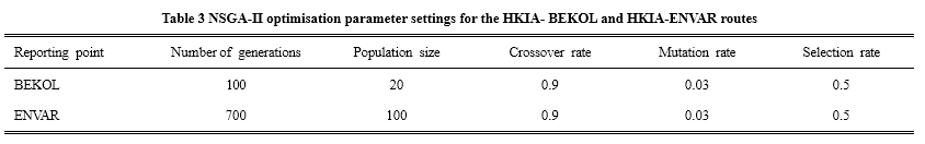
1. Hong Kong to London
The altitude paths from HKIA to BEKOL are shown on the left-hand side of Fig 9, and the corresponding fuel consumption and accumulated perceived noise level are shown on the right-hand side. The accumulated noise level here corresponds only to the climb segment as mentioned in Sec. II.B.3. The take-off weight of the aircraft is set as 3XX,XXX kg (masked for confidentiality reasons, as stipulated in the agreement with our airline partner), which is the average based on QAR data. The computational models for fuel consumption and accumulated perceived noise level are validated by comparison against QAR data used in this study. The relative errors of fuel consumption and accumulated perceived noise level are 4.10 and 2.34% respectively, which provide sufficient accuracy for the optimisations in this study.
As shown on the left-hand side of Fig 9, the results satisfy the travel distances of Dubins and PA*S paths from the surface path planning presented in Table 2, at the end of the take-off and accelerated climb segments respectively. The trajectories of the generated altitude paths are quite similar to QAR paths. On the right-hand side, the distributions of fuel consumption and perceived noise level values are shown as colour-coded circles for simulation results (i.e., solutions generated from the NSGA-II optimisation), and those for QAR paths are shown as purple stars. The altitude path plots show a significantly wider distribution of altitudes corresponding to simulation results compared to those of QAR paths. Note, however, that the total distances to BEKOL vary in actual flights, as observed at the end-points of the QAR paths, unlike the simulation results. The notable altitude variations from the simulation results and the flight distance variations from the QAR paths yield similar ranges of fuel consumption distributions (approximately 300 kg), although the distribution for the QAR paths is located closer to the right, indicating higher fuel consumption.
Table 4 shows the altitude at the ATS reporting point corresponding to the Pareto front set shown on the right-hand side in Fig 9, along with their corresponding fuel consumption and accumulated perceived noise levels. The noise-minimum path has a target altitude of 15,458 feet. This is depicted on the right-hand side of Fig 9 as the magenta triangle at the bottom. The corresponding path is depicted on the left-hand side of Fig 9, which has a final altitude lower than those of the QAR paths. The fuel-minimum path has a target altitude of 18,917 feet. This is depicted on the right-hand side of Fig 9 as the magenta triangle at the left. The corresponding path is depicted on the left-hand side of Fig 9, which has a final altitude higher than those of the QAR paths. In the case of noise level, we observe that the colour, in general, transitions from yellow to dark blue as the value of the vertical axis on the right figure increases, which indicates that the noise level increases as the target altitude increases. This trend is caused by the higher engine power output needed to climb to the increased target altitude, which correspondingly affects the perceived noise level. However, this trend reverses when the target altitude is around 16,400 feet, where a set of greenish circles can be observed near the noise-minimum point below a set of yellowish circles. For the paths in this specific region, i.e., where the noise trend reverses, the aircraft increases its lift force to reach the higher altitude not by increasing the engine power, but by adjusting the angle of attack or high lift device deployment. Hence the noise level, which is primarily a function of engine power and distance in our model, can be decreased with a similar engine power level and a higher distance from the ground. Similarly, the colour changes from yellow to dark blue as the value of the horizontal axis increases, which indicates that fuel consumption increases as the target altitude increases. However, more careful analysis reveals that the highest fuel consumption occurs at the highest altitude, whereas the lowest fuel consumption does not correspond to the lowest altitude. The turning point occurs at an altitude around 19,000 feet, near the fuel-minimum point. The Pareto front lies near this turning point, verifying the optimisation results. We note that the cardinality of the Pareto front set may be small as the design space is restricted by the prescribed interval used to generate the discrete design variables.
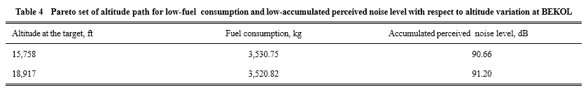
2. Hong Kong to Taipei
The altitude paths from HKIA to ENVAR are shown at the top of Fig 10, and the corresponding fuel consumption and accumulated perceived noise levels with the design variables are shown at the bottom. The accumulated perceived noise level here also corresponds only to the climb segments. The take-off weight of the aircraft is set as 2XX,XXX kg (masked for confidentiality reasons), which is the average based on QAR data. The path plot at the top shows that the travel distance of Dubins path at the end of take-off and the travel distances of PA*S at the end of the accelerated climb and constant Mach number cruise segments are satisfied.
The figure shows that the feasible take-off altitude paths generated by the simulations are almost identical to the QAR paths, and that the variation of QAR paths during take-off is small. The major difference occurs near the end of take-off, where most of the QAR paths maintain level flight for a short period before the subsequent climbing stage, which is not considered in our altitude path formulation. Despite this difference in modelling, most of the QAR paths are still within the operational bounds of the feasible solutions generated in the optimisation (the light blue region). We observe that the climb angles of the respective QAR paths sharply increase after this short level-flight phase. In this phase, the paths follow a similar pattern to the solutions with a high climb rate, which are also similar to the paths of the Pareto front set. This pattern deviates to two altitudes at the end of the climb phase: cruise at approximately 37,000 feet and approximately 35,000 feet. These are also within the operational bounds of the solutions, and the Pareto front set is distributed near the latter cruise altitude.
The distributions of the three discretised design variables (cruise Mach number, altitude at transition point, and altitude at target) and their impact on the objective functions (fuel consumption and accumulated perceived noise level) are shown at the bottom of Fig 10. The horizontal axes of the first three columns from the left show the design variable domains, and the last two columns show the objective function ranges. The vertical axes of the two rows from the top represent cruise Mach number and target altitude, and the last two rows represent objectives. Graphs at the top of each column are histograms. The three histograms along the diagonal represent the distributions of the samples generated in the design space, and of their outputs in the last two. The distributions of the design variables generated are mostly uniform during the optimisation, except for the target altitude near the upper bound. From the first column, we observe that the discrete cruise Mach number and discrete altitude at the target are generated with a constant interval. We also observe that the fuel consumption and accumulated perceived noise levels decrease as the altitude at the transition point increases. The Pareto front is concentrated to the right side of the graphs in the first column, indicating that the optimal set is near the upper bound of the altitude at the transition point corresponding to higher climb angles, which is also observed in the path plots of Fig 10 (top). The Pareto front is concentrated to the left side of the graphs in the third column, indicating that the optimal set is near the lower bound of the target altitude. From the fourth column, we observe that noise level tends to increase as fuel consumption increases. The Pareto front is listed in Table 5, with the fuel-minimum and noise-minimum solutions indicated in bold. We observe a negligible difference in noise level between the two, but a notable difference in fuel consumption with higher fuel consumed at the lower Mach number 0.8. This is attributed to the design cruise speed of the 777-300ER being approximately 0.84, which is the reference for the aircraft used in this study. The ranges of fuel consumption and accumulated perceived noise level in the optimisation are presented in Table 6 to highlight the effects of the developed optimisation problem formulations. The Solutions column in Table 6 refers to all solutions evaluated in the optimisation process, and the Pareto front column refers to the set of optimal choices among them. The fuel and noise ranges of the Pareto front are much lower than those of the solutions, even though the noise range of solutions for BEKOL and the fuel range of solutions for ENVAR are large. This implies that any of the Pareto front choices, which constitutes an optimum solution without determining a prior preference, do not result in any significant trade-off between minimum fuel consumption and perceived noise levels.
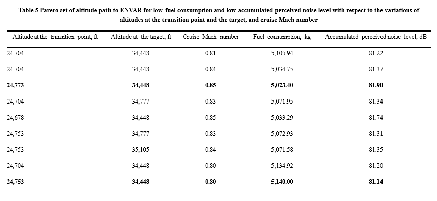
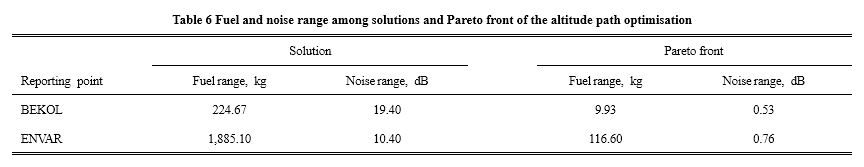
IV. Conclusions
This paper presents a flight path optimisation methodology for low-fuel consumption and low-accumulated perceived noise levels along a flight path during departure. The methodology is developed for generating a set of four-dimensional departure paths for an aircraft flying from an airport to the compulsory ATS reporting point, considering flight destination, runway angles, spatial separation near an airport, obstacles, populated regions, and steering, to support the decision-making processes of SID planning, flight planners, and pilots. The developed strategy performs surface path planning and altitude path planning sequentially. The former generates the shortest path consisting of initial and subsequent departure paths. Dubins path is applied to determine the initial departure path satisfying constraints of runway angles and spatial separation directions. The population-aware A* with steering constraints algorithm is developed to perform path planning for the subsequent departure path satisfying constraints pertaining to obstacles, populated regions, and steering motions. Altitude paths are generated by solving the longitudinal governing equations of motion of flight. The accumulated perceived noise level and fuel consumption along the paths are computed using the ANP database and performance parameters obtained from evaluating flight dynamics. The nondominated set of fuel consumption and noise level points of the altitude paths is obtained by applying multi-objective optimisation using a modified NSGA-II for discrete optimisation. A study is conducted on the path planning for an aircraft similar to a Boeing 777-300ER with GE90-115B engines using the developed methodology in two flight scenarios departing from Hong Kong International Airport (HKIA). The population-aware A* with steering constraints method yields a path with close similarity to the Standard Instrument Departure (SID) tracks and certain Quick Access Recorder (QAR) paths by graphical comparison. The multi-objective optimisation results show that the trends of fuel and noise level reductions depend on the altitude at the transition point of upper flight level, Mach number, and altitude at the compulsory ATS reporting point. Furthermore, the optimisation yields a small cluster of optimal solutions with less than 120 kg variation in fuel consumption and 0.8 dB variation in perceived noise. The methodology can be further used to analyse flight paths, and extended to unmanned aerial vehicle and urban air mobility path planning, especially with complex air transportation-related constraints and multiple criteria for decision making. Although we have implemented realistic constraints in the flight operations departing from HKIA, we have not considered air traffic interactions and weather conditions in this research. By extending this study to include such factors, we can perform more comprehensive departure route coordination and optimisation around HKIA. By including the relevant constraints, the method can also be generalised to make it applicable to other airports.
Acknowledgments
This work is supported by the Hong Kong University of Science and Technology (HKUST) Start-Up Grant (Project No. R9354) and Research Support from Chau Hoi Shuen Foundation. The authors would like to thank Cathay Pacific Airways Limited for providing the data used in this study under the Data Partnership Agreement between the airline and the Department of Mechanical and Aerospace Engineering, HKUST. The authors would also like to thank Young-jong Lee from Seoul regional aviation office and Raymond Li from the Civil Aviation Department in Hong Kong for their helpful advice on this research, and Arjit Seth for his diligent proofreading. The authors additionally thank the anonymous reviewers of this paper for their constructive feedback and helpful suggestions.
References:
- Mahashabde, A., Wolfe, P., Ashok, A., Dorbian, C., He, Q., Fan, A., Lukachko, S., Mozdzanowska, A., Wollersheim, C., Barrett, S. R., et al., "Assessing the Environmental Impacts of Aircraft Noise and Emissions," Progress in Aerospace Sciences, Vol. 47, No. 1, 2011, pp. 15–52. https://doi.org/10.1016/j.paerosci.2010.04.003
- Ho-Huu, V., Hartjes, S., Visser, H., and Curran, R., "Integrated Design and Allocation of Optimal Aircraft Departure Routes," Transportation Research Part D: Transport and Environment, Vol. 63, Aug. 2018, pp. 689–705. https://doi.org/10.1016/j.trd.2018.07.006
- Bertsch, L., and Isermann, U., "Noise Prediction Toolbox Used by the DLR Aircraft Noise Working Group," INTER-NOISE the 42nd International Congress and Exposition on Noise Control Engineering, Vol. 247, Inst. of Noise Control Engineering, Reston, VA, 2013, pp. 805–813, https://www.researchgate.net/profile/Lothar-Bertsch/publication/257773363_Noise_prediction_toolbox_used_by_the_DLR_aircraft_noise_working_group/links/00b49525d6a02d5634000000/Noise-prediction-toolbox-used-by-the-DLR-aircraft-noise-working-group.pdf
- Casalino, D., Diozzi, F., Sannino, R., and Paonessa, A., "Aircraft Noise Reduction Technologies: A Bibliographic Review," Aerospace Science and Technology, Vol. 12, No. 1, 2008, pp. 1–17. https://doi.org/10.1016/j.ast.2007.10.004
- Ho-Huu, V., Hartjes, S., Pérez-Castán, J., Visser, H., and Curran, R., "A Multilevel Optimization Approach to Route Design and Flight Allocation Taking Aircraft Sequence and Separation Constraints into Account," Transportation Research Part C: Emerging Technologies, Vol. 117, Aug. 2020, Paper 102684. https://doi.org/10.1016/j.trc.2020.102684
- Kim, D., Lyu, Y., and Liem, R. P., "Flight Profile Optimization for Noise Abatement and Fuel Efficiency During Departure and Arrival of an Aircraft," AIAA Aviation 2019 Forum, AIAA Paper 2019-3622, 2019. https://doi.org/10.2514/6.2019-3622
- Patrón, R. S. F., Botez, R. M., and Labour, D., "Vertical Profile Optimization for the Flight Management System CMA-9000 Using the Golden Section Search Method," IECON 2012-38th Annual Conference on IEEE Industrial Electronics Society, Inst. of Electrical and Electronics Engineers, New York, 2012, pp. 5482–5488. https://doi.org/10.1109/IECON.2012.6389517
- "Procedure for Air Navigation Services (PANS)—Aircraft Operations," Procedure, International Civil Aviation Organization, Montreal, 2018, https://store.icao.int/en/procedures-for-air-navigation-services-pans-aircraft-operations-volume-i-flight-procedures-doc-8168
- Zachary, D. S., Gervais, J., and Leopold, U., "Multi-Impact Optimization to Reduce Aviation Noise and Emissions," Transportation Research Part D: Transport and Environment, Vol. 15, No. 2, 2010, pp. 82–93. https://doi.org/10.1016/j.trd.2009.09.005
- Prats, X., Puig, V., Quevedo, J., and Nejjari, F., "Multi-Objective Optimisation for Aircraft Departure Trajectories Minimising Noise Annoyance," Transportation Research Part C: Emerging Technologies, Vol. 18, No. 6, 2010, pp. 975–989. https://doi.org/10.1016/j.trc.2010.03.001
- Torres, R., Chaptal, J., Bès, C., and Hiriart-Urruty, J.-B., "Optimal, Environmentally Friendly Departure Procedures for Civil Aircraft," Journal of Aircraft, Vol. 48, No. 1, 2011, pp. 11–22. https://doi.org/10.2514/1.C031012
- Ho-Huu, V., Hartjes, S., Visser, H. G., and Curran, R., "An Efficient Application of the MOEA/D Algorithm for Designing Noise Abatement Departure Trajectories," Aerospace, Vol. 4, No. 4, Nov. 2017, pp. 1–15. https://doi.org/10.3390/aerospace4040054
- Filippone, A., Zhang, M., and Bojdo, N., "Validation of an Integrated Simulation Model for Aircraft Noise and Engine Emissions," Aerospace Science and Technology, Vol. 89, June 2019, pp. 370–381. https://doi.org/10.1016/j.ast.2019.04.008
- Thomas, J., and Hansman, R. J., "Evaluation of the Impact of Transport Jet Aircraft Approach and Departure Speed on Community Noise," Massachusetts Inst. of Technology, Cambridge, MA, 2020, https://rosap.ntl.bts.gov/view/dot/56957
- Chai, R., Savvaris, A., Tsourdos, A., Xia, Y., and Chai, S., "Solving Multiobjective Constrained Trajectory Optimization Problem by an Extended Evolutionary Algorithm," IEEE Transactions on Cybernetics, Vol. 50, No. 4, 2018, pp. 1630–1643. https://doi.org/10.1109/TCYB.2018.2881190
- Kant, K., and Zucker, S. W., "Toward Efficient Trajectory Planning: The Path-Velocity Decomposition," International Journal of Robotics Research, Vol. 5, No. 3, 1986, pp. 72–89. https://doi.org/10.1177/027836498600500304
- Hartjes, S., and Visser, H., "Efficient Trajectory Parameterization for Environmental Optimization of Departure Flight Paths Using a Genetic Algorithm," Proceedings of the Institution of Mechanical Engineers, Part G: Journal of Aerospace Engineering, Vol. 231, No. 6, 2017, pp. 1115–1123. https://doi.org/10.1177/0954410016648980
- Zhang, Y., Zhang, R., and Li, H., "Graph-Based Path Decision Modeling for Hypersonic Vehicles with No-Fly Zone Constraints," Aerospace Science and Technology, Vol. 116, Sept. 2021, Paper 106857. https://doi.org/10.1016/j.ast.2021.106857
- Zhang, Z., Du, R., and Cowlagi, R. V., "Randomized Sampling-Based Trajectory Optimization for UAVs to Satisfy Linear Temporal Logic Specifications," Aerospace Science and Technology, Vol. 96, Jan. 2020, Paper 105591. https://doi.org/10.1016/j.ast.2019.105591
- Qian, K., Liu, Y., Tian, L., and Bao, J., "Robot Path Planning Optimization Method Based on Heuristic Multi-Directional Rapidly-Exploring Tree," Computers & Electrical Engineering, Vol. 85, July 2020, Paper 106688. https://doi.org/10.1016/j.compeleceng.2020.106688
- Li, Z., Yang, X., Sun, X., Liu, G., and Hu, C., "Improved Artificial Potential Field Based Lateral Entry Guidance for Waypoints Passage and No-Fly Zones Avoidance," Aerospace Science and Technology, Vol. 86, March 2019, pp. 119–131. https://doi.org/10.1016/j.ast.2019.01.015
- Wang, H., and Pan, W., "Research on UAV Path Planning Algorithms," IOP Conference Series: Earth and Environmental Science, Vol. 693, IOP Publ., Bristol, England, U.K., 2021, Paper 012120, https://iopscience.iop.org/article/10.1088/1755-1315/693/1/012120/pdf
- Haghighi, H., Asadi, D., and Delahaye, D., "Multi-Objective Cooperated Path Planning of Multiple UAVs Based on Revisit Time," Journal of Aerospace Information Systems, Vol. 18, No. 12, 2021, pp. 1–14. https://doi.org/10.2514/1.I010866
- Heidari, H., and Saska, M., "Collision-Free Trajectory Planning of Multi-Rotor UAVs in a Wind Condition Based on Modified Potential Field," Mechanism and Machine Theory, Vol. 156, Feb. 2021, Paper 104140. https://doi.org/10.1016/j.mechmachtheory.2020.104140
- Guo, J., Li, B., and Ji, Y., "A Control Parametrization Based Path Planning Method for the Quad-Rotor UAVs," Journal of Industrial & Management Optimization, Vol. 13, No. 5, March 2021, pp. 1079–1100. https://doi.org/10.3934/jimo.2021009
- Huang, Y., Chen, J., Wang, H., and Su, G., "A Method of 3D Path Planning for Solar-Powered UAV with Fixed Target and Solar Tracking," Aerospace Science and Technology, Vol. 92, Sept. 2019, pp. 831–838. https://doi.org/10.1016/j.ast.2019.06.027
- Abd Algfoor, Z., Sunar, M. S., and Kolivand, H., "A Comprehensive Study on Pathfinding Techniques for Robotics and Video Games," International Journal of Computer Games Technology, Vol. 2015, April 2015, Paper 736138. https://doi.org/10.1155/2015/736138
- Kavraki, L., and Latombe, J. C., "Randomized Preprocessing of Configuration Space for Path Planning: Articulated Robots," Proceedings of IEEE/RSJ International Conference on Intelligent Robots and Systems (IROS’94), Vol. 3, Inst. of Electrical and Electronics Engineers, New York, 1994, pp. 1764–1771. https://doi.org/10.1109/IROS.1994.407619
- Karaman, S., and Frazzoli, E., "Sampling-Based Algorithms for Opti-mal Motion Planning," International Journal of Robotics Research, Vol. 30, No. 7, 2011, pp. 846–894. https://doi.org/10.1177/0278364911406761
- Andrews, J. R., "Impedance Control as a Framework for Implementing Obstacle Avoidance in a Manipulator," Master's Thesis, Dept. of Mechanical Engineering, Massachusetts Inst. of Technology, Cambridge, MA, 1983.
- Koren, Y., and Borenstein, J., "Potential Field Methods and Their Inherent Limitations for Mobile Robot Navigation," Proceedings of 1991 IEEE International Conference on Robotics and Automation, Vol. 2, April 1991, pp. 1398–1404. https://doi.org/10.1109/ROBOT.1991.131810
- Betts, J. T., "Survey of Numerical Methods for Trajectory Optimization," Journal of Guidance, Control, and Dynamics, Vol. 21, No. 2, 1998, pp. 193–207. https://doi.org/10.2514/2.4231
- Petereit, J., Emter, T., Frey, C. W., Kopfstedt, T., and Beutel, A., "Application of Hybrid A* to an Autonomous Mobile Robot for Path Planning in Unstructured Outdoor Environments," ROBOTIK 2012; 7th German Conference on Robotics, Verband Deutscher Elektrotech-niker (VDE), May 2012, pp. 1–6, https://ieeexplore.ieee.org/document/6309512
- The Defence Mapping Agency (DMA) World Geodetic System 84 Development Committee, "Department of Defense World Geodetic System 1984: Its Definition and Relationships with Local Geodetic Systems," United States Defense Mapping Agency TR 8350.2, Sept. 1991, https://ia800106.us.archive.org/29/items/DTIC_ADA280358/DTIC_ADA280358.pdf
- "Aeronautical Information Manual," Federal Aviation Administration, 2008, https://www.faa.gov/air_traffic/publications/atpubs/aim_html/chap1_section_2.html
- McGrath, C. N., and Macdonald, M., "General Perturbation Method for Satellite Constellation Reconfiguration Using Low-Thrust Maneuvers," Journal of Guidance, Control, and Dynamics, Vol. 42, No. 8, 2019, pp. 1676–1692. https://doi.org/10.2514/1.G003739
- Dubins, L. E., "On Curves of Minimal Length with a Constraint on Average Curvature, and with Prescribed Initial and Terminal Positions and Tangents," American Journal of Mathematics, Vol. 79, No. 3, 1957, pp. 497–516, https://www.jstor.org/stable/2372560
- Jha, B., Chen, Z., and Shima, T., "On Shortest Dubins Path via a Circular Boundary," Automatica, Vol. 121, Nov. 2020, Paper 109192. https://doi.org/10.1016/j.automatica.2020.109192
- Hart, P. E., Nilsson, N. J., and Raphael, B., "A Formal Basis for the Heuristic Determination of Minimum Cost Paths," IEEE Trans- actions on Systems Science and Cybernetics, Vol. 4, No. 2, 1968, pp. 100–107. https://doi.org/10.1109/TSSC.1968.300136
- Deb, K., Pratap, A., Agarwal, S., and Meyarivan, T., "A Fast and Elitist Multiobjective Genetic Algorithm: NSGA-II," IEEE Transactions on Evolutionary Computation, Vol. 6, No. 2, 2002, pp. 182–197. https://doi.org/10.1109/4235.996017
- Mailund, T., "Divide and Conquer and Dynamic Programming," Introduction to Computational Thinking, Springer, New York, 2021, pp. 247–288. https://doi.org/10.1007/978-1-4842-7077-6_9
- Kim, D., Seth, A., and Liem, R. P., "Data-Enhanced Dynamic Flight Simulations for Flight Performance Analysis," Aerospace Science and Technology, Vol. 121, Feb. 2022, Paper 107357. https://doi.org/10.1016/j.ast.2022.107357
- "Standard Atmosphere," ISO/TC 20/SC 6, International Organization for Standardization, Geneva, 1975, https://www.iso.org/standard/7472.html
- Polhamus, E. C., A Simple Method of Estimating the Subsonic Lift and Damping in Roll of Sweptback Wings, Vol. 1862, NACA, 1949, https://ntrs.nasa.gov/citations/19930082534
- Dubs, F., "ProfIlform und Polare," Aerodynamik der reinen Unterschallströmung, Vol. 1, Springer, Berlin, 2013, pp. 167–235. https://doi.org/10.1007/978-3-0348-5295-1
- Jahanmiri, M., "Aircraft Drag Reduction: An Overview," Chalmers Univ. of Technology, Gothenburg, Sweden, 2011, https://publications.lib.chalmers.se/records/fulltext/137214.pdf
- Bouhlel, M. A., Hwang, J. T., Bartoli, N., Lafage, R., Morlier, J., and Martins, J. R. R. A., "A Python Surrogate Modeling Framework with Derivatives," Advances in Engineering Software, Vol. 135, Sept. 2019, Paper 102662. https://doi.org/10.1016/j.advengsoft.2019.03.005
- The Society of Automotive Engineers (SAE) A-21 Aircraft Noise Measure and Noise Aviation Emission Modeling Committee, "Procedure for the Calculation of Airplane Noise in the Vicinity of Airports," Society of Automotive Engineers, Aerospace Information Rept. 1845, Sept. 1995. https://doi.org/10.4271/AIR1845
- European Civil Aviation Conference (ECAC), "Report on Standard Method of Computing Noise Contours Around Civil Airports," Euro-pean Civil Aviation Conference, ECAC.CEAC Doc 29, 2016, https://www.ecac-ceac.org/images/documents/ECAC-Doc_29_4th_edition_Dec_2016_Volume_1.pdf
- Boeker, E. R., Dinges, E., He, B., Fleming, G., Roof, C. J., Gerbi, P. J., Rapoza, A. S., Hermann, J., et al., "Integrated Noise Model (INM) Version 7.0 Technical Manual," United States Federal Aviation Administration Office of Environment and Energy, 2008, https://www.faa.gov/about/office_org/headquarters_offices/apl/research/models/inm_model/inm7_0c/media/INM_7.0_Technical_Manual.pdf
Footnotes:
‡ https://www.ais.gov.hk
¶ https://www.ais.gov.hk
§ https://earth.google.com
** www.cad.gov.hk/english/ac_path.html
†† https://sedac.ciesin.columbia.edu/data/set/gpw-v4-admin-unit-center-points-population-estimates-rev11/data-download
‡‡ https://www.aircraftnoisemodel.org/
Authors:
Prof Rhea P Liem, Assistant Professor, Department of Mechanical and Aerospace Engineering, The Hong Kong University of Science and Technology
Dr Dajung Kim, Postdoctoral Researcher, The Hong Kong University of Science and Technology
Associate Editor:
I-Hwang
Presented as Paper 2019-3622 at the AIAA Aviation 2019 Forum, Dallas, TX, June 17–21, 2019; received 3 January 2022; revision received 22 May 2022; accepted for publication 25 July 2022; published online 27 September 2022. Copyright © 2022 by the American Institute of Aeronautics and Astronautics, Inc. All rights reserved. All requests for copying and permission to reprint should be submitted to CCC at www.copyright.com; employ the eISSN 1533-385X to initiate your request. See also AIAA Rights and Permissions www.aiaa.org/randp.
March 2023