A powerful mathematical modeling tool---phase field method

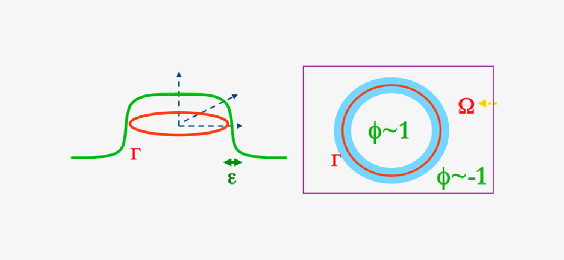
The idea of the phase field method could be traced back to Lord Rayleigh, Josiah Willard Gibbs and Van der Waals. Since then, it has emerged as a powerful approach for modeling and predicting mesoscale morphological and microstructural evolution arising from many fields, such as biology, material sciences, image processing, multiphase fluid mechanics, chemical and petroleum engineering, etc. A variety of phase field models have been derived to describe phase separations and transitions. In general, phase field models take distinct values (for instance, +1 and -1 in Fig 1) in each of the phases, with a smooth change between phase values in a thin layer of finite width around the interface.

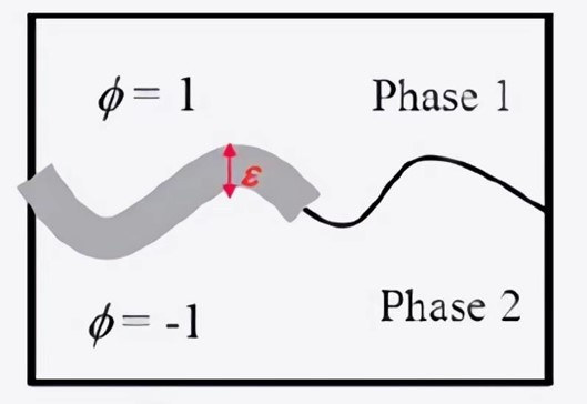
Fig 1. Phase field function

Energy functionals play an important role in the phase field method. In the phase field approach, phase separations and transitions processes are energy driven in the sense that the dynamics is the gradient flow of a certain Helmholtz energy functional. The Helmholtz free energy functional can be written as the sum of two parts: the interfacial energy and the bulk energy. The interfacial energy measures the energy stored in the interfacial layer and can be defined with the help of the phase function (ϕ in Fig 1). As expected, it would depend on the width of the interfacial layer (ε in Fig 1). On the other hand, the bulk energy is usually problem dependent and may consist of several other types of energies such as kinetic and potential/gradient energy. This energetic approach makes the phase field modeling become systematic. In practice, the main task of the phase field modeling is the construction of the Helmholtz free energy functional and the driving forces that provide the mechanism of energy dissipation.

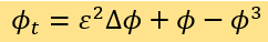
The Allen-Cahn equation

(1)

and the Cahn-Hilliard equation

(2)

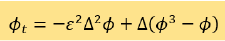
are two best known phase field equations, which are and gradient flows of the following Helmholtz energy functional, respectively:

(3)

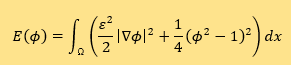
Here, is the interfacial energy density and is the bulk energy density, which is a popular-used double-well potential. The small positive parameter ε measures the width of the diffuse interface layer.

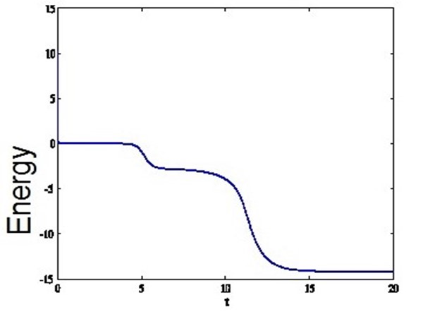
Fig 2. Energy dissipation

Effective numerical methods for phase field models

After a phase field model is obtained, how to solve it efficiently and accurately becomes a crucial problem. To design effective numerical methods in simulations, several important issues must be considered. First, an intrinsic property of phase field equations is that energy functionals decay in time, i.e.,

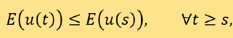
which is often called energy stability. In order to preserve the gradient flow structure at the discrete level, it is desirable to ensure the numerical method to be energy stable besides to be accurate, which is a non-trivial task, especially if one aims to have high order schemes in time. In this past decade, many energy stable time integration methods have been developed and successfully used in various of phase field simulations. Preserving, on the discrete level, other physical features associated with the continuum phase field dynamics (such as uniform pointwise bounds on the phase field variable for the Allen-Cahn equation) has also taken increasingly attention in the literature. The readers could refer to [2,7] and the references therein for related numerical analysis. Second, in order to resolve the thin interfacial layer, one must use spatial mesh sizes that are much smaller than the layer width ε for computer simulations (note that ε <<1). For such extremely small mesh sizes, the resulting large linear and nonlinear algebraic problems require huge computational effort to solve. This is especially true in the three-dimensional case with uniform spatial meshes. To overcome the difficulty, one may use adaptive methods that only use fine meshes in the interfacial layer and much coarser meshes away from the layer. The use of adaptive mesh is a natural choice considering the fact that the phase function has a nice, structured profile that assumes distinct (close-to-constant) values in bulk phases away from the diffuse interface and has a large gradient in the diffuse interface. Finally, it usually takes a long-time simulation to reach the steady state of the phase field equation, while at different stage, the decay rate of the Helmholtz energy functional may vary significantly. See Fig 2 for the discrete energy dissipation of a Cahn-Hilliard simulation. A natural idea is to use small time steps when energy decays rapidly and large time steps otherwise. [5] gives an adaptive strategy, which is very easy to implement in practice. The formulation is given by

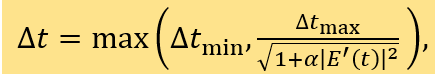
where is the Helmholtz energy functional defined in the phase field model. The constant α is used to adjust the level of the adaptivity. The pre-set smallest time step is to force the adaptive time steps bounded from below to avoid too small time steps. Likewise, gives the upper bound of the time steps.

Applications

Simulating the time evolution of phase field models has many important applications such as phase transition, microstructure coarsening and cell motion. With different selections of the Helmholtz free energy functionals, various phase field models have been developed and simulated for complex phenomena, such as dendritic crystal growth, alloy solidification, multiphase flows, liquid crystal, tumor growth, etc. Among them, many models couple phase field equations and other physical models, for instance, Cahn-Hilliard-Navier-Stokes equations and Cahn-Hilliard-Microelasticity models. To character the uncertainty nature of phase separation and transition, stochastic phase field models, such as stochastic Allen-Cahn and Cahn-Hilliard equations, are also widely studied in the literature. Fig 3 gives a simulation for the evolution of macromolecular microsphere composite hydrogels with random force effect in polymer mixture systems. Most recently, the phase field method has become an effective approach in the imaging segmentation (See Fig 4 for image segmentations of ‘tiger in the lake’ and ‘cameraman’) and classification of high dimensional data. Readers can refer to [1] for a review.

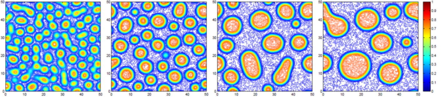
Fig 3. Macromolecular microsphere composite hydrogels [3]

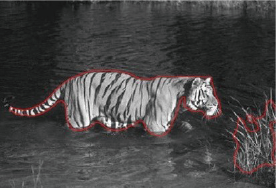
Fig 4. Image segmentation [4]

Conclusions

The phase field method is an effective mathematical approach for solving interfacial problems. In applications, phase field models can be developed by constructing different Helmholtz free energy functionals. Computer simulations play an important role in the study of phase field models. There have been increasingly interests in developing highly stable and efficient numerical schemes for solving phase field models. Numerical simulations of phase field models remain to be challenging, especially in high dimensions, because of sheer amount of computations involved. Indeed, phase field simulations on extreme scales have been used as a test of computing power on world’s leading high performance computers as exemplified by the appearances on the Gordon Bell prize competition [6] (2011 Gordon Bell prize winner) and [8] (2016 Gordon Bell prize finalist, which reported the largest 3D phase field simulations to date that reached 40 Petaflops on the world’s fastest supercomputer at the time, employing over 300 billion spatial grid points and utilising over 10 million cores). With the increasing popularity of phase field modeling in more and more applications, it is imperative that efficient numerical algorithms and solvers such as adaptive grid methods, adaptive time-stepping strategies and parallel techniques must be developed and utilised.

References

1. Bertozzi A. L. and Flenner A. Diffuse interface models on graphs for classification of high dimensional data. SIAM Review, 2016, 58: 293-328.
2. Du Q and Feng X. The phase field method for geometric moving interfaces and their numerical approximations, in Geometric Partial Differential Equations, Handbook of Numerical Analysis, 2020, 21: 425-508.
3. Li X, Qiao Z and Zhang H. A second-order convex splitting scheme for a Cahn-Hilliard equation with variable interfacial parameters. J. Comput. Math., 2017, 35: 693-710.
4. Liu C, Qiao Z and Zhang Q. Efficient numerical methods of the Allen-Cahn intensity fitting model for image segmentation. In preparation, 2020.
5. Takashi S, Takayuki A, Tomohiro T, Akinori Y, Akira N, Toshio E, Naoya M, Satoshi M, and Malcolm C. Peta-scale phase-field simulation for dendritic solidification on the Tsubame 2.0 supercomputer. In Proceedings of 2011 International Conference for High Performance Computing, Networking, Storage and Analysis (SC ’11). Article No. 3, 2011.
6. Tang T and Qiao Z. Efficient numerical methods for phase-field equations (in Chinese). Sci. Sin. Math., 2020, 50: 775-794.
7. Qiao Z, Zhang Z and Tang T. An adaptive time-stepping strategy for the molecular beam epitaxy models. SIAM J Sci Comput., 2011, 33: 1395-1414.
8. Zhang J, Zhou C, Wang Y, Ju L, Du Q, Chi X, Xu D, Chen D, Liu Y, and Liu Z. Extreme-scale phase field simulations of coarsening dynamics on the Sunway TaihuLight supercomputer. In Proceedings of the International Conference for High Performance Computing, Networking, Storage and Analysis, page 4. IEEE Press, 2016.

Author:
Prof Zhonghua QIAO
Professor, Department of Applied Mathematics
The Hong Kong Polytechnic University

January 2020