We introduced the International Mathematical Modeling Challenge (IM2C) in “Science in the Community”. It is an innovative contest in mathematical modeling for secondary school students all over the world. With the help of IM2C Committee (Zhonghua) and participating schools, we are pleased to share one of the topics (Smart Water Data Analysis) for the 2020 Greater China contest and a corresponding winning paper.
Water is essential in our daily life, an effective transport system of water is extremely crucial for the benefits of users. However, in a water supply system, water leaks may easily be caused by system malfunctions, for example, flaws in water pipes and valves, such high vulnerability is always a big problem. Engineers and researchers are constantly exploring the methods of constructing a smart water system so as to use water efficiently. Thus, electromagnetic flowmeters are often used for water flow measurement and leak monitoring. For example, the difference of the input water flow and the output water flow in a given region can be analysed in detail so that the flow status and leak potentials can be reviewed clearly. Although many data analysis methods are available nowadays, some challenges still exist. International Mathematical Modeling Challenge (IM2C) sets such challenge for secondary school students from Greater China.
To feature all IM2C problems coming from real world, this problem is created by experts of Hong Kong Applied Science and Technology Research Institute (ASTRI) from their real project. The original problem and its dataset containing the data of the difference of the input water flow and the output water flow in 8 different virtual regions could be found here.
The article below is abbreviated from the winning paper by Diocesan Girls’ School in Hong Kong which has won Outstanding Award in IM2C 2020 of Greater China.
If you are secondary school students or you are teaching in secondary school, and interested in participating in the challenge, please stay tuned here for the latest information.
Students: Lam Wai Sum, So Wing Tung Abby, Wong Ka Yu, Yu Sui Ki Rita
Teacher Advisor: Yeung Po Ki Dora
The data pattern is first observed and the criteria for identifying the abnormality from the given data is determined. It is observed that the data in all 8 regions generally fluctuates quite a lot and there is no obvious regular pattern. However, the difference between the water input and water output (referred as actual values) remains from -12 to 24. The small fluctuations are considered to be created due to the slight change in people’s water usage everyday, while the large fluctuations are caused by abnormalities in water flow.
As a set of data of the difference of input and output water flow in 8 different regions is provided, 8 model functions are calculated according to their corresponding data sets, which are applicable to only that region. Through these model functions, the trend of water flow in each region can be predicted, and so as the detection of abnormal water flow and leakage. The R2 value measures how accurate our model function is with respect to the actual data. If R2 > 0.5, it is considered as a good model. The closer the value is to 1, the better the model. Since the R2 values of all 8 regions are less than 0.5, it shows that the data distribution in all 8 regions is very dispersed, there is no direct relationship between the data.
The first criteria for abnormality considers the actual values of each day. Points exceeding the normal range by 5% are classified as abnormal and are considered as serious water leakage problems that can be detected in a very short period of time.
The second criteria for abnormality considers the magnitude of change of the actual values every 5 days through calculating the average slope of 5 consecutive actual values from the dataset. Points with an average slope that exceeds the normal slope range by 5% are considered as abnormal. The actual individual points considered may not have exceeded the normal range yet, but the water leakage may accumulate and worsen, which could lead to serious water leakage in the future if left unattended.
Afterwards, a general mathematical model to do abnormal detection for the 8 virtual regions based on the result of data analysis is developed.
The first approach is to find the normal range of actual values.
Firstly, the centered moving average of the given data is calculated. (Let the actual value of day x be Ax.) The first and last 7 moving averages (i.e. 1st-7th, 94th-100th day) are calculated separately since there is insufficient data for it to be the median of 15 days. Otherwise, the moving average of day x is calculated by ( Ax-7 + Ax-6 + ... + Ax + Ax+6 + Ax+7 ) / 15 . The first 7 moving averages are calculated by ( A1 + A2 + A3 + ... + A2x-1 ) / ( 2x -1 ) ; and the last seven moving averages by ( A2x-100 + ... + A98 + A99 + A100 ) / ( 201 - 2x ) .
Then, the moving variance is found using this formula:
Moving Variance = moving average of (actual value(x) - average of actual values)2
The moving standard deviation is the square root of the moving variance:
Moving Standard Deviation = square root of Moving Variance
Upper Limit = Moving average of actual value + 2 x Moving Standard Deviation
Lower Limit = Moving average of actual value - 2 x Moving Standard Deviation
Below is an example of the graph of normal range produced from the given data in Region 7:
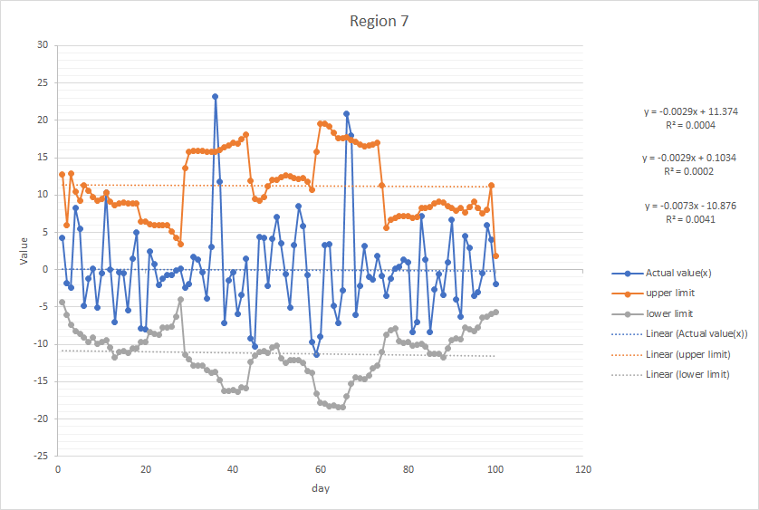
The Moving Standard Deviation is multiplied by 2 since it includes around 95% of the data, which implies that about 5% of the data is not in the range, of which are considered as abnormal. Since there are different moving averages in different regions, the Moving Standard Deviations are different in respect of their corresponding data and water flow situation and are calculated separately.
Moving average allows us to analyse the trend of data instead of analyzing each data separately. This is useful because there is a need to compare the data with each other to determine whether the water flow is considered as abnormal. The trend of water flow in the future can also be forecasted. A longer period for calculating moving average is used (i.e. 15 days per interval), which can smooth out short-term fluctuations and highlight longer-term trends to simplify calculations. Furthermore, using an odd number interval eases the checking process. It is only required to find the number in the middle of the set of data and see if it differentiates from the calculated average a lot, which helps decrease the possibility of having abnormalities.
Moving averages can be calculated using the simple or cumulative moving average method. However, the former one is chosen because this only takes the recent data as a reference, which can help spot the sudden abnormality more easily. Whereas the latter method takes the data from the first day. The cumulative moving average of day x (CMAx) is calculated by ( A1 + A2 + ... + Ax ) / x , where the actual value of day x is indicated by Ax. While the cumulative moving average of day x + 1 is calculated by ( Ax+1 + x(CMAx)) / ( x+1 ) . If there is an abnormal point in the dataset, it may not be realised as quickly due to the large amount of data taken into consideration. Therefore, when a point is found to be abnormal, it might not always be the case, instead it might be because of an accumulated effect of multiple abnormal data added previously. As the number of days is an even number, 100, a definite midpoint does not exist. Therefore, the centered simple moving average method is used, which adds a layer of averaging atop the moving averages, which smoothens the calculated moving averages and produces a midpoint for them.
The second approach is to calculate the normal slope range of the data.
Each slope on the graph illustrates the change of difference between the water input and output over a certain number of days. Thus, it shows a change of water output when the points differ from the previous one, since the water input is consistent. Therefore, the slope can be used to measure the magnitude of the increase or decrease in water output. As mentioned above, when the average slope of 5 consecutive points which are located above the model function of the actual values of that region is greater than the normal range, which is calculated by the simple standard deviation, it is considered as a large sudden decrease of total water output, and vice versa.
5 consecutive points are chosen to calculate since if too few points are considered, there will be inaccuracies in determining whether there is an abnormality in the water flow due to noise factors, for example, a malfunction of the electromagnetic flowmeter. Meanwhile, if too many points are considered, the efficiency of detecting abnormal water leakage problems will be lowered, making it unable to send warning signals before the issue turns serious. Therefore, 5 points are considered.
To calculate the normal slope range, the average slope is first found between every 5 consecutive points, then the average of those values is calculated. Then, the variance of the values is found using this formula:
Variance = average of (actual value - average of actual values)2
Next, the simple standard deviation is calculated by taking the square root of the variance. The range of the slope is then calculated using these formulae:
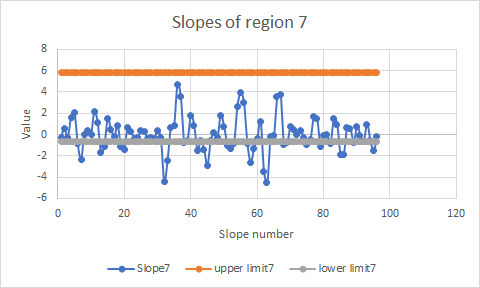
Upper Limit of Normal Slope Range = Average of actual slope values + 2 x Simple Standard Deviation
Lower Limit of Normal Slope Range = Average of actual slope values - 2 x Simple Standard Deviation
Similar to moving standard deviation, simple standard deviation has to be multiplied twice so that it covers 95% of the data which is normal. The remaining 5% is considered abnormal.
Below is an example of the graph of normal slope range produced from the given data in Region 7:
After fully developing the mathematical model, a comparison is done between the two approaches. The normal range is calculated using the moving average method, which reduces the influence of noise, including the malfunction of electromagnetic flowmeter. (The amount of noise reduction is square root of 15, which is the square root of the number of points we used in our calculation of the centered moving average). Abnormalities can also be detected more quickly.
Whereas the method of normal slope range is calculated by simple standard deviation, which takes less time and can detect more abnormalities, so more minor mistakes can be detected which will alert people more often and prevent problems in the future.
The data of all 8 regions is stored into an excel file and used python programming to check the abnormalities so that numbers that are needed can be calculated easily. The usage of python allows abnormal points to be found more quickly and clearly. After inputting the given data into our programme, results for days with abnormal water flow due to the actual value exceeding the normal range and due to the slope of actual values exceeding the normal slope range are generated.
After developing the mathematical model and testing our model based on the given data, a self-evaluation on our model is done.
One strength of this mathematical model is that it allows people to detect abnormality of water flow more efficiently and effectively since the electromagnetic flowmeters can send signals to the water supply system immediately once it detects any water flow abnormality. This can allow people to repair water pipes or the water supply system as soon as possible so that the worsening of water leakage can be prevented.
Another strength is that it is very user friendly and easy to use. All that is required is to download the Excel file and input the region number, then the abnormal points in the data set can be found. This allows people to identify the water leakage problem in a short period of time, which further increases the efficiency and effectiveness of letting the water supply system be back to normal.
Last but not least, this model detects abnormal water flow by using two approaches: using the normal range and using the normal slope range. These two approaches detect major problems of water leakage and minor leak potentials respectively. By using both approaches, the abnormality of water flow can be detected in a more comprehensive way.
However, a limitation of this model is that it cannot detect the abnormal water flow in smaller water pipe branches since the difference of water input and water output of those water pipes is insignificant due to the large population in each region. Therefore, it neglects the problem of water leakage in smaller water pipe branches.
In conclusion, a mathematical model is developed, with the ability to understand many flowmeters’ data patterns simultaneously and detect the abnormality of the flowing effectively and efficiently. The data pattern is analysed and the criteria for identifying the abnormality from the given data is figured out. A general mathematical model to do abnormal detection for the 8 virtual regions based on the result of data analysis is developed. Our model is tested based on the given dataset and a logical explanation of our modeling and the result of abnormal detection is provided. We hope to tackle the serious problem of water leakage faced by the general public, by warning the water supplier and the general public of the abnormal water flow and preventing the leak potentials to turn into a serious water leakage problem.
Reference:
- Variance: Simple Definition, Step by Step Examples https://www.statisticshowto.datasciencecentral.com/probability-and-statistics/variance/
- Standard Deviation https://www.statisticshowto.datasciencecentral.com/probability-and-statistics/variance/
- What is R-squared https://www.displayr.com/what-is-r-squared/
- Bell Curve and Normal Distribution Definition https://www.thoughtco.com/bell-curve-normal-distribution-defined-2312350
- Moving Average https://www.investopedia.com/terms/m/movingaverage.asp
- Calculating standard deviation step by step https://www.khanacademy.org/math/statistics-probability/summarizing-quantitative-data/variance-standard-deviation-population/a/calculating-standard-deviation-step-by-step
- Moving Averages and Simple Moving Averages http://www.informit.com/articles/article.aspx?p=2433607&seqNum=2
- Cumulative Moving Average https://qkdb.wordpress.com/2013/05/11/cumulative-moving-average/
- Calculating standard deviation step by step https://www.khanacademy.org/math/statistics-probability/summarizing-quantitative-data/variance-standard-deviation-population/a/calculating-standard-deviation-step-by-step
- Moving Averages and Centered Moving Averages https://www.mathsisfun.com/data/standard-deviation.html
- Standard Deviation and Variance https://www.mathsisfun.com/data/standard-deviation.html
- Bell Curve and Normal Distribution Definition https://www.thoughtco.com/bell-curve-normal-distribution-defined-2312350
- Moving Average Filters https://www.analog.com/media/en/technical-documentation/dsp-book/dsp_book_Ch15.pdf
July 2020